Julia and partial differential equations

Using the example of the most typical physical models, we will consolidate the skills of working with functions and become familiar with the fast, convenient and beautiful PyPlot visualizer, which provides all the power of the Python Matplotlib. There will be a lot of pictures (hidden under spoilers)

Make sure everything under the hood is clean and fresh:

Under the hood

]status Status `C:\Users\\.julia\environments\v1.0\Project.toml` [537997a7] AbstractPlotting v0.9.0 [ad839575] Blink v0.8.1 [159f3aea] Cairo v0.5.6 [5ae59095] Colors v0.9.5 [8f4d0f93] Conda v1.1.1 [0c46a032] DifferentialEquations v5.3.1 [a1bb12fb] Electron v0.3.0 [5789e2e9] FileIO v1.0.2 [5752ebe1] GMT v0.5.0 [28b8d3ca] GR v0.35.0 [c91e804a] Gadfly v1.0.0+ #master (https://github.com/GiovineItalia/Gadfly.jl.git) [4c0ca9eb] Gtk v0.16.4 [a1b4810d] Hexagons v0.2.0 [7073ff75] IJulia v1.13.0+ [`C:\Users\\.julia\dev\IJulia`] [6218d12a] ImageMagick v0.7.1 [c601a237] Interact v0.9.0 [b964fa9f] LaTeXStrings v1.0.3 [ee78f7c6] Makie v0.9.0+ #master (https://github.com/JuliaPlots/Makie.jl.git) [7269a6da] MeshIO v0.3.1 [47be7bcc] ORCA v0.2.0 [58dd65bb] Plotly v0.2.0 [f0f68f2c] PlotlyJS v0.12.0+ #master (https://github.com/sglyon/PlotlyJS.jl.git) [91a5bcdd] Plots v0.21.0 [438e738f] PyCall v1.18.5 [d330b81b] PyPlot v2.6.3 [c4c386cf] Rsvg v0.2.2 [60ddc479] StatPlots v0.8.1 [b8865327] UnicodePlots v0.3.1 [0f1e0344] WebIO v0.4.2 [c2297ded] ZMQ v1.0.0

Otherwise, we are pumping everything we need for today.

 julia>] pkg> add PyCall pkg> add LaTeXStrings pkg> add PyPlot pkg> build PyPlot #     build #    -      ,    pkg> add Conda #    Jupyter -    pkg> add IJulia #      pkg> build IJulia #     build

Now to the tasks!

Transport equation

In physics, the term transfer means irreversible processes, as a result of which spatial displacement (transfer) of mass, momentum, energy, charge, or some other physical quantity occurs in a physical system.
A linear one-dimensional transport equation (or advection equation) —the simplest partial differential equation — is written as

$\ frac {\ partial U (x, t)} {\ partial t} + c \ frac {\ partial U (x, t)} {\ partial x} = \ Phi (U, x, t)$

For the numerical solution of the transport equation, an explicit difference scheme can be used:

$\ frac {\ hat {U} _i-U_i} {\ tau} + c \ frac {U_i-U_ {i-1}} {\ Delta} = \ frac {\ Phi_ {i-1} + \ Phi_i} {2}$

Where $\ hat {U}$ - the value of the grid function on the upper time layer. This scheme is stable with the Courant number. $K = c \ tau / \ Delta <1$

Nonlinear transfer

$\ frac {\ partial U (x, t)} {\ partial t} + (C_0 + UC_1) \ frac {\ partial U (x, t)} {\ partial x} = \ Phi (U, x, t )$

Line source (absorption transfer): $\ Phi (U, x, t) = - BU$ . We use the explicit difference scheme:

$U ^ {j + 1} _i = \ left (1- \ frac {h_tB} {2} - \ frac {h_tC_0} {h_x} - \ frac {h_tC_1} {h_x} U ^ j_i \ right) U ^ j_i + U ^ j_ {i-1} \ left (\ frac {h_tC_0} {h_x} - \ frac {h_tB} {2} + \ frac {h_tC_1} {h_x} U ^ j_i \ right)$

 using Plots pyplot() a = 0.2 b = 0.01 ust = x -> x^2 * exp( -(xa)^2/b ) #   bord = t -> 0. #  #    - function transferequi(;C0 = 1., C1 = 0., B = 0., Nx = 50, Nt = 50, tlmt = 0.01) dx = 1/Nx dt = tlmt/Nt b0 = 0.5B*dt c0 = C0*dt/dx c1 = C1*dt/dx print("Kurant: $c0 $c1") x = [i for i in range(0, length = Nx, step = dx)]#         t = [i for i in range(0, length = Nt, step = dt)] #   -   U = zeros(Nx, Nt) U[:,1] = ust.(x) U[1,:] = bord.(t) for j = 1:Nt-1, i = 2:Nx U[i, j+1] = ( 1-b0-c0-c1*U[i,j] )*U[i,j] + ( c0-b0+c1*U[i,j] )*U[i-1,j] end t, x, U end t, X, Ans0 = transferequi( C0 = 4., C1 = 1., B = 1.5, tlmt = 0.2 ) plot(X, Ans0[:,1], lab = "t1") plot!(X, Ans0[:,10], lab = "t10") p = plot!(X, Ans0[:,40], lab = "t40") plot( p, heatmap(t, X, Ans0) ) #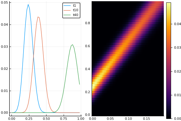

Result

Strengthen absorption:

 t, X, Ans0 = transferequi( C0 = 2., C1 = 1., B = 3.5, tlmt = 0.2 ) plot(X, Ans0[:,1]) plot!(X, Ans0[:,10]) p = plot!(X, Ans0[:,40]) plot( p, heatmap(t, X, Ans0) )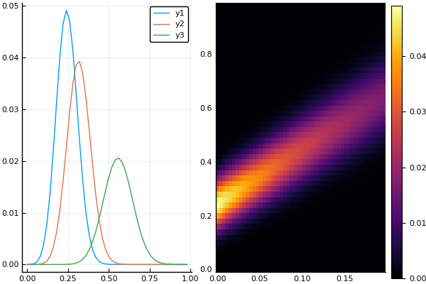

Result

 t, X, Ans0 = transferequi( C0 = 1., C1 = 15., B = 0.1, Nx = 100, Nt = 100, tlmt = 0.4 ) plot(X, Ans0[:,1]) plot!(X, Ans0[:,20]) plot!(X, Ans0[:,90])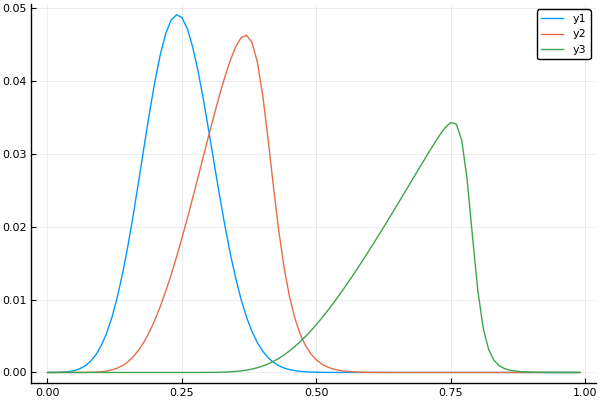

Almost knocked over

heatmap(t, X, Ans0)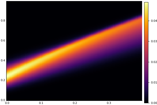

Heat equation

The differential heat equation (or the heat diffusion equation) is written as follows:

$\ frac {\ partial T (x, t)} {\ partial t} + D \ frac {\ partial ^ 2 U (x, t)} {\ partial x ^ 2} = \ phi (T, x, t )$

This equation is of parabolic type, containing the first derivative with respect to time t and the second with respect to the spatial coordinate x. It describes the temperature dynamics, for example, of a cooling or heated metal rod (the function T describes the temperature profile along the x-coordinate along the rod). The coefficient D is called the coefficient of thermal conductivity (diffusion). It can be either constant or depend, either explicitly on the coordinates, or on the desired function D (t, x, T) itself.

Consider a linear equation (diffusion coefficient and heat sources do not depend on temperature). Difference approximation of a differential equation using an explicit and implicit Euler scheme, respectively:

$\ frac {T_ {i, n + 1} -T_ {i, n}} {\ tau} = D \ frac {T_ {i-1, n} -2T_ {i, n} + T_ {i + 1 , n}} {\ Delta ^ 2} + \ phi_ {i, n} \\ \ frac {T_ {i, n + 1} -T_ {i, n}} {\ tau} = D \ frac {T_ { i-1, n + 1} -2T_ {i, n + 1} + T_ {i + 1, n + 1}} {\ Delta ^ 2} + \ phi_ {i, n}$

 δ(x) = x==0 ? 0.5 : x>0 ? 1 : 0 # -     startcond = x-> δ(x-0.45) - δ(x-0.55) #   bordrcond = x-> 0. #    D(u) = 1 #   Φ(u) = 0 #    #      LaTex    Tab # \delta press Tab -> δ function linexplicit(Nx = 50, Nt = 40; tlmt = 0.01) dx = 1/Nx dt = tlmt/Nt k = dt/(dx*dx) print("Kurant: $k dx = $dx dt = $dt k<0.5? $(k<0.5)") x = [i for i in range(0, length = Nx, step = dx)] #         t = [i for i in range(0, length = Nt, step = dt)] #   -   U = zeros(Nx, Nt) U[: ,1] = startcond.(x) U[1 ,:] = U[Nt,:] = bordrcond.(t) for j = 1:Nt-1, i = 2:Nx-1 U[i, j+1] = U[i,j]*(1-2k*D( U[i,j] )) + k*U[i-1,j]*D( U[i-1,j] ) + k*U[i+1,j]*D( U[i+1,j] ) + dt*Φ(U[i,j]) end t, x, U end t, X, Ans2 = linexplicit( tlmt = 0.005 ) plot(X, Ans2[:,1], lab = "t1") plot!(X, Ans2[:,10], lab = "t10") p = plot!(X, Ans2[:,40], lab = "t40", title = "Explicit scheme") plot( p, heatmap(t, X, Ans2) )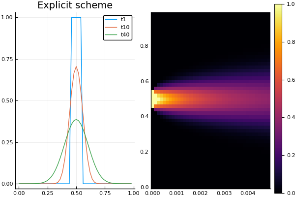

Result

We use the implicit scheme and the method of sweep.

 function nonexplicit(Nx = 50, Nt = 40; tlmt = 0.01) dx = 1/Nx dt = tlmt/Nt k = dt/(dx*dx) print("Kurant: $k dx = $dx dt = $dt k<0.5? $(k<0.5)\n") x = [i for i in range(0, length = Nx, step = dx)] t = [i for i in range(0, length = Nt, step = dt)] U = zeros(Nx, Nt) η = zeros(Nx+1) ξ = zeros(Nx) U[: ,1] = startcond.(x) U[1 ,:] = bordrcond.(t) U[Nt,:] = bordrcond.(t) for j = 1:Nt-1 b = -1 - 2k*D( U[1,j] ) c = -k*D( U[2,j] ) d = U[1,j] + dt*Φ(U[1,j]) ξ[2] = c/b η[2] = -d/b for i = 2:Nx-1 a = -k*D( U[i-1,j] ) b = -2k*D( U[i,j] ) - 1 c = -k*D( U[i+1,j] ) d = U[i,j] + dt*Φ(U[i,j]) ξ[i+1] = c / (ba*ξ[i]) η[i+1] = (a*η[i]-d) / (ba*ξ[i]) end U[Nx,j+1] = η[Nx] for i = Nx:-1:2 U[i-1,j+1] = ξ[i]*U[i,j+1] + η[i] end end t, x, U end plot(X, Ans2[:,1], lab = "ex_t1") plot!(X, Ans2[:,10], lab = "ex_t10") plot!(X, Ans2[:,40], lab = "ex_t40") plot!(X, Ans3[:,1], lab = "non_t1") plot!(X, Ans3[:,10], lab = "non_t10") plot!(X, Ans3[:,40], lab = "non_t40", title = "Comparison schemes")

Comparison schemes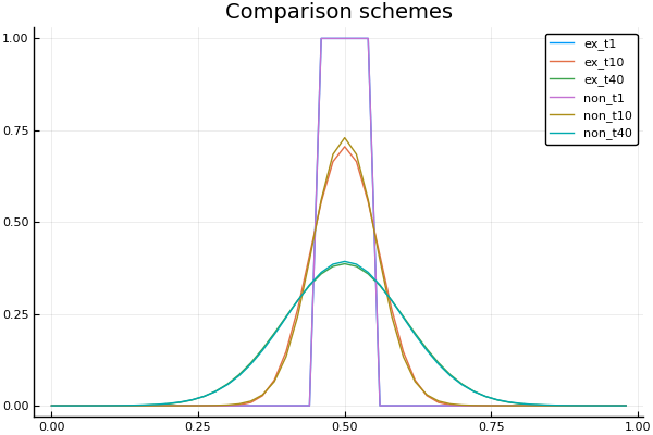

Nonlinear heat equation

Much more interesting solutions can be obtained for a nonlinear heat equation, for example, with a nonlinear heat source. $\ phi (x, T) = 10 ^ 3 (T-T ^ 3)$ . If you set it in this form, then you get a solution in the form of thermal fronts that propagate in both directions from the primary heating zone

 Φ(u) = 1e3*(uu^3) t, X, Ans4 = linexplicit( tlmt = 0.005 ) plot(X, Ans4[:,1], lab = "ex_t1") plot!(X, Ans4[:,10], lab = "ex_t10") plot!(X, Ans4[:,40], lab = "ex_t40", title = "Thermal front")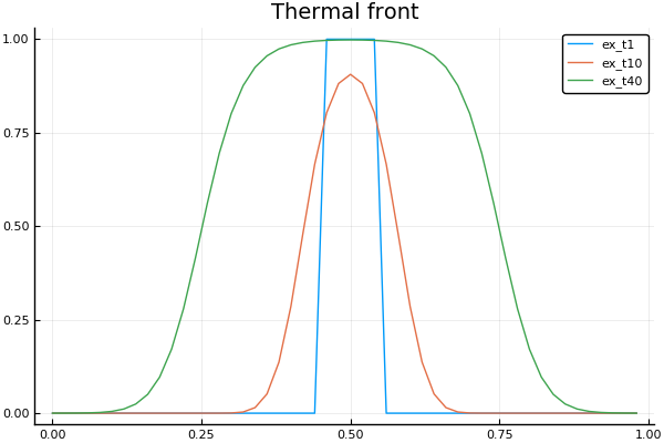

Thermal front

Even more unexpected solutions are possible with nonlinearity and also the diffusion coefficient. For example, if you take $D (x, T) = T ^ 2$ a $\ phi (x, T) = 10 ^ 3T ^ {3.5}$ , then we can observe the effect of burning environment, localized in the area of its primary heating (S-mode of combustion "with exacerbation").
At the same time let's check how our implicit scheme works with nonlinearity and sources and diffusion coefficient

 D(u) = u*u Φ(u) = 1e3*abs(u)^(3.5) t, X, Ans5 = linexplicit( tlmt = 0.0005 ) t, X, Ans6 = nonexplicit( tlmt = 0.0005 ) plot(X, Ans5[:,1], lab = "ex_t1") plot!(X, Ans5[:,10], lab = "ex_t10") p1 = plot!(X, Ans5[:,40], lab = "ex_t40", title = "Burning with aggravation") p2 = heatmap(abs.(Ans6-Ans5), title = "Difference") #      plot(p1, p2)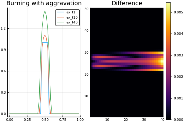

S-mode

Wave equation

Wave equation of hyperbolic type

$\ frac {\ partial ^ 2 U (x, t)} {\ partial t ^ 2} = c ^ 2 \ frac {\ partial ^ 2 U (x, t)} {\ partial x ^ 2}$

describes one-dimensional linear waves without dispersion. For example, string vibrations, sound in a liquid (gas), or electromagnetic waves in a vacuum (in the latter case, the equation should be written in vector form).

The simplest difference scheme that approximates this equation is the explicit five-point scheme.

$\ frac {U ^ {n + 1} _i-2U ^ {n} _i + U ^ {n-1} _i} {\ tau ^ 2} = c ^ 2 \ frac {U ^ n_ {i + 1} -2U ^ n_i + U ^ n_ {i-1}} {h ^ 2} \\ x_i = ih, \, t_n = \ tau$

This scheme, called the “cross”, has the second order of accuracy in time and spatial coordinate and is three-layer in time.

 #     ψ = x -> x^2 * exp( -(x-0.5)^2/0.01 ) #    ϕ(x) = 0 c = x -> 1 #     function pdesolver(N = 100, K = 100, L = 2pi, T = 10, a = 0.1 ) dx = L/N; dt = T/K; gam(x) = c(x)*c(x)*a*a*dt*dt/dx/dx; print("Kurant-Fridrihs-Levi: $(dt*a/dx) dx = $dx dt = $dt") u = zeros(N,K); x = [i for i in range(0, length = N, step = dx)] #      u[:,1] = ψ.(x); u[:,2] = u[:,1] + dt*ψ.(x); #     fill!( u[1,:], 0); fill!( u[N,:], ϕ(L) ); for t = 2:K-1, i = 2:N-1 u[i,t+1] = -u[i,t-1] + gam( x[i] )* (u[i-1,t] + u[i+1,t]) + (2-2*gam( x[i] ) )*u[i,t]; end x, u end N = 50; #     K = 40; #    a = 0.1; #    L = 1; #   T = 1; #   t = [i for i in range(0, length = K, stop = T)] X, U = pdesolver(N, K, L, T, a) #    plot(X, U[:,1]) plot!(X, U[:,40])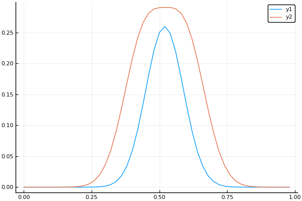

Result

To build a surface, we will use PyPlot not as an environment of Plots, but directly:

Graphic surface

 using PyPlot surf(t, X, U)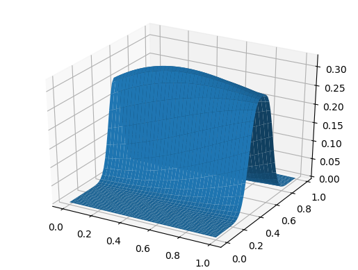

And for dessert, wave propagation at a speed dependent on the coordinate:

 ψ = x -> x>1/3 ? 0 : sin(3pi*x)^2 c = x -> x>0.5 ? 0.5 : 1 X, U = pdesolver(400, 400, 8, 1.5, 1) plot(X, U[:,1]) plot!(X, U[:,40]) plot!(X, U[:,90]) plot!(X, U[:,200], xaxis=("  ", (0, 1.5), 0:0.5:2) )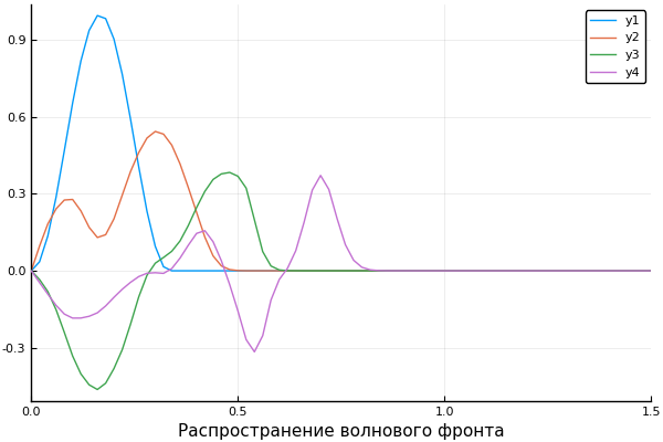

Result

 U2 = [ U[i,j] for i = 1:60, j = 1:size(U,2) ] #    surf(U2) #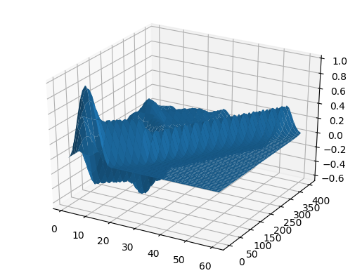

heatmap(U, yaxis=(" ", (0, 50), 0:10:50))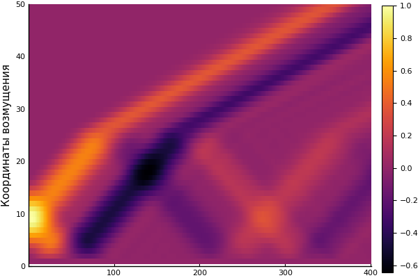

It's enough for today. For more detailed information:
PyPlot reference to githabs , more examples of using Plots as an environment, and a good Russian-language Julia memo .

Source: https://habr.com/ru/post/429218/

All Articles

Julia and partial differential equations

Transport equation

Nonlinear transfer

Heat equation

Nonlinear heat equation

Wave equation

More articles: