Overview of the main mathematical optimization methods for problems with constraints
I have been preparing and collecting material for a long time, I hope this time turned out better. This article is dedicated to the main methods of solving mathematical optimization problems with constraints, so if you have heard that the simplex method is a very important method, but you still do not know what it does, then this article may help you.
PS The article contains mathematical formulas added by the macro editor. They say that they are sometimes not displayed. There are also many animations in gif format.
The task of mathematical optimization is a task of the “Find in a set element such that for all of performed "That in the scientific literature it will most likely be written down somehow
Historically, popular methods such as gradient descent or Newton's method work only in linear spaces (and preferably simple, for example ). In practice, there are often problems where you need to find a minimum in a non-linear space. For example, you need to find the minimum of some function on such vectors for which This may be due to the fact that denote the length of any objects. Or for example, if represent the coordinates of the point that should be at a distance no more from i.e. . For such tasks, gradient descent or Newton's method is not directly applicable. It turned out that a very large class of optimization problems is conveniently covered by “constraints”, similar to those I described above. In other words, it is convenient to represent the set in the form of a system of equalities and inequalities
Minimization tasks over a view space thus, they became conditionally called “problems without constraints” (the unconstrained problem), and tasks over sets defined by sets of equalities and inequalities - “problems with constraints” (constrained problem).
Technically, absolutely any set can be represented as a single equality or inequality using the indicator function, which is defined as
However, such a function does not have different useful properties (convexity, differentiability, etc.). However, you can often imagine in the form of several equalities and inequalities, each of which has such properties. The main theory is brought under the case
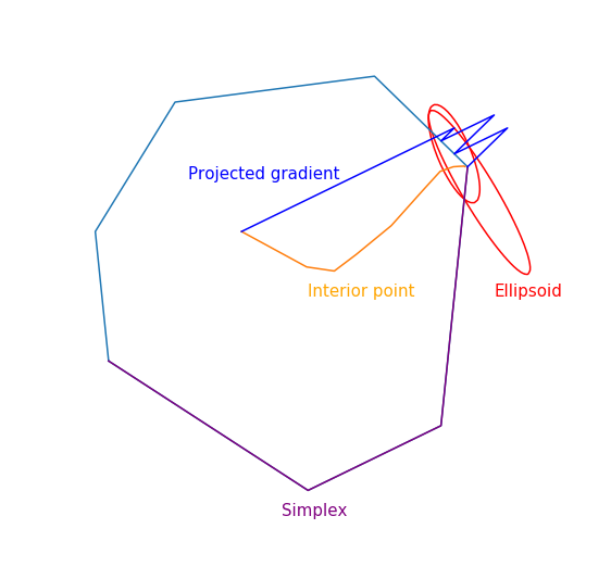
Where - convex (but not necessarily differentiable) functions, - matrix. To demonstrate how the methods work, I will use two examples:
')
Of all the methods that I cover with this review, the simplex method is probably the most famous. The method was developed specifically for linear programming and the only one presented achieves an exact solution in a finite number of steps (provided that exact arithmetic is used for calculations, in practice this is usually not the case, but in theory it is possible). The idea of the simplex method consists of two parts:
The simplex method is iterative, that is, it consistently improves the solution slightly. For such methods, you need to start somewhere, in general, this is done by solving auxiliary problem
If to solve this problem such that then executed otherwise, the original problem is generally given on the empty set. To solve an auxiliary problem, you can also use the simplex method, the starting point can be with arbitrary . Finding the starting point can be called the first phase of the method, finding the solution to the original problem can be called the second phase of the method.
I recently wrote a separate article about gradient descent, in which I also briefly described this method. Now this method is quite lively, but is being studied as part of a more general proximal gradient descent . The very idea of the method is completely trivial: if we apply a gradient descent to a convex function then, with the right choice of parameters, we get the global minimum . If, after each step of the gradient descent, the resulting point is corrected, instead of taking its projection onto the closed convex set then as a result we get the minimum of the function on . Well or more formally, a projective gradient descent is an algorithm that sequentially calculates
Where
The last equation defines a standard projection operator on a set; in fact, it is a function that, by the point computes the nearest point of the set . The role of distance plays here It is worth noting that any norm can be used here, however, projections with different norms may differ!
In practice, projective gradient descent is used only in special cases. Its main problem is that the calculation of the projection can be even more challenging than the original, and it needs to be calculated many times. The most common case for which it is convenient to apply a projective gradient descent is “boxed constraints”, which have the form
In this case, the projection is calculated very simply, for each coordinate is obtained
The use of projective gradient descent for linear programming problems is completely meaningless; nevertheless, if you do this, it will look something like this.
But what does the projective gradient descent trajectory look like for the second task, if
and if
This method is remarkable because it is the first polynomial algorithm for linear programming problems; it can be considered a multidimensional generalization of the bisection method . I will start with a more general method of separating hyperplanes :
For optimization problems, the construction of a “separating hyperplane” is based on the following inequality for convex functions
If fix , then for a convex function half space contains only points with a value not less than at a point , which means they can be cut off, since these points are no better than the one we have already found. For problems with constraints, you can likewise get rid of points that are guaranteed to violate any of the constraints.
The simplest version of the separating hyperplane method is to simply cut off half-spaces without adding any points. As a result, at each step we will have a certain polyhedron. The problem with this method is that the number of faces of a polyhedron is likely to increase from step to step. Moreover, it can grow exponentially.
The ellipsoid method actually stores an ellipsoid at every step. More precisely, after the hyperplane, an ellipsoid of minimal volume is constructed, which contains one of the parts of the original one. This is achieved by adding new points. An ellipsoid can always be defined by a positive definite matrix and vector (the center of the ellipsoid) as follows
The construction of a minimum volume ellipsoid containing the intersection of a half-space and another ellipsoid can be accomplished using moderately cumbersome formulas . Unfortunately, in practice, this method was still not as good as the simplex method or the interior point method.
But actually how it works for
and for
This method has a long history of development, one of the first prerequisites appeared around the same time as the simplex method was developed. But at that time it was not yet sufficiently effective to be used in practice. Later in 1984, a variant of the method was developed specifically for linear programming, which was good both in theory and in practice. Moreover, the internal point method is not limited only to linear programming, unlike the simplex method, and now it is the main algorithm for convex optimization problems with constraints.
The basic idea of the method is the replacement of restrictions on the penalty in the form of the so-called barrier function . Function called the barrier function for the set , if a
Here - the inside , - the border . Instead, the original problem is proposed to solve the problem.
and set only on the inside (essentially hence the name), the barrier property ensures that at least exists. Moreover, the more the greater the impact . Under sufficiently reasonable conditions, one can achieve that if one strives to infinity then the minimum will converge to the solution of the original problem.
If many specified as a set of inequalities , the standard choice of the barrier function is the logarithmic barrier
Minimum points functions for different forms a curve, which is usually called the central path , the method of the inner point as if trying to follow this path. That's what it looks like for
Finally, the internal point method itself has the following form.
The use of Newton's method is very important here: the fact is that with the right choice of the barrier function, the step of Newton's method generates a pointthat remains inside our set , experimented, does not always produce this form. Finally, the trajectory of the inner point method
PS The article contains mathematical formulas added by the macro editor. They say that they are sometimes not displayed. There are also many animations in gif format.
Preamble
The task of mathematical optimization is a task of the “Find in a set element such that for all of performed "That in the scientific literature it will most likely be written down somehow
Historically, popular methods such as gradient descent or Newton's method work only in linear spaces (and preferably simple, for example ). In practice, there are often problems where you need to find a minimum in a non-linear space. For example, you need to find the minimum of some function on such vectors for which This may be due to the fact that denote the length of any objects. Or for example, if represent the coordinates of the point that should be at a distance no more from i.e. . For such tasks, gradient descent or Newton's method is not directly applicable. It turned out that a very large class of optimization problems is conveniently covered by “constraints”, similar to those I described above. In other words, it is convenient to represent the set in the form of a system of equalities and inequalities
Minimization tasks over a view space thus, they became conditionally called “problems without constraints” (the unconstrained problem), and tasks over sets defined by sets of equalities and inequalities - “problems with constraints” (constrained problem).
Technically, absolutely any set can be represented as a single equality or inequality using the indicator function, which is defined as
However, such a function does not have different useful properties (convexity, differentiability, etc.). However, you can often imagine in the form of several equalities and inequalities, each of which has such properties. The main theory is brought under the case
Where - convex (but not necessarily differentiable) functions, - matrix. To demonstrate how the methods work, I will use two examples:
- Linear programming task
$$ display $$ \ begin {array} {rl} \ mbox {minimize} & -2 & x ~~~ - & y \\ \ mbox {provided} & -1.0 & ~ x -0.1 & ~ y \ leq -1.0 \ \ & -1.0 & ~ x + ~ 0.6 & ~ y \ leq -1.0 \\ & -0.2 & ~ x + ~ 1.5 & ~ y \ leq -0.2 \\ & ~ 0.7 & ~ x + ~ 0.7 & ~ y \ leq 0.7 \\ & ~ 2.0 & ~ x -0.2 & ~ y \ leq 2.0 \\ & ~ 0.5 & ~ x -1.0 & ~ y \ leq 0.5 \\ & -1.0 & ~ x -1.5 & ~ y \ leq - 1.0 \\ \ end {array} $$ display $$
In essence, this task is to find the farthest point of the polygon in the direction (2, 1), the solution to the problem is the point (4.7, 3.5) - the most “right” in the polygon). But actually the polygon itself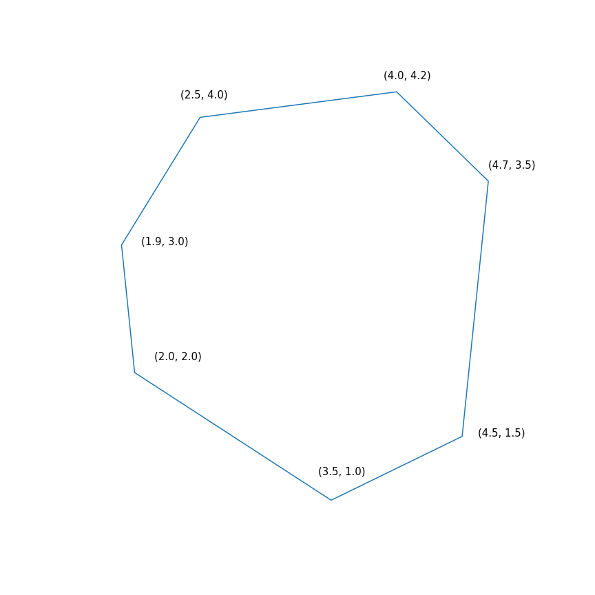
- Minimization of a quadratic function with a single quadratic constraint
')
Simplex method
Of all the methods that I cover with this review, the simplex method is probably the most famous. The method was developed specifically for linear programming and the only one presented achieves an exact solution in a finite number of steps (provided that exact arithmetic is used for calculations, in practice this is usually not the case, but in theory it is possible). The idea of the simplex method consists of two parts:
- Systems of linear inequalities and equalities define multidimensional convex polytopes (polytopes). In the one-dimensional case, it is a point, a ray, or a segment, in a two-dimensional one, a convex polygon, and in a three-dimensional case, a convex polyhedron. Minimizing a linear function is essentially finding the furthest point in a certain direction. I think intuition should suggest that there should be some peak at this furthest point, and this is indeed so. In general, for a system of inequalities in -dimensional space a vertex is a point satisfying a system for which exactly of these inequalities turn into equalities (provided that among the inequalities there are no equivalent). There are always a finite number of such points, although there may be a lot of them.
- Now we have a finite set of points, generally speaking, you can simply pick them up, that is, to do something like this: for each subset of inequalities to solve a system of linear equations constructed on the selected inequalities, verify that the solution fits into the original system of inequalities and compare with other such points. This is a rather simple, inefficient, but working method. The simplex method instead of iteration moves from vertex to vertex along edges so that the values of the objective function are improved. It turns out that if a vertex has no “neighbors” in which the function values are better, then it is optimal.
The simplex method is iterative, that is, it consistently improves the solution slightly. For such methods, you need to start somewhere, in general, this is done by solving auxiliary problem
If to solve this problem such that then executed otherwise, the original problem is generally given on the empty set. To solve an auxiliary problem, you can also use the simplex method, the starting point can be with arbitrary . Finding the starting point can be called the first phase of the method, finding the solution to the original problem can be called the second phase of the method.
The trajectory of the two-phase simplex method
The trajectory was generated using scipy.optimize.linprog.
Projective Gradient Descent
I recently wrote a separate article about gradient descent, in which I also briefly described this method. Now this method is quite lively, but is being studied as part of a more general proximal gradient descent . The very idea of the method is completely trivial: if we apply a gradient descent to a convex function then, with the right choice of parameters, we get the global minimum . If, after each step of the gradient descent, the resulting point is corrected, instead of taking its projection onto the closed convex set then as a result we get the minimum of the function on . Well or more formally, a projective gradient descent is an algorithm that sequentially calculates
Where
The last equation defines a standard projection operator on a set; in fact, it is a function that, by the point computes the nearest point of the set . The role of distance plays here It is worth noting that any norm can be used here, however, projections with different norms may differ!
In practice, projective gradient descent is used only in special cases. Its main problem is that the calculation of the projection can be even more challenging than the original, and it needs to be calculated many times. The most common case for which it is convenient to apply a projective gradient descent is “boxed constraints”, which have the form
In this case, the projection is calculated very simply, for each coordinate is obtained
The use of projective gradient descent for linear programming problems is completely meaningless; nevertheless, if you do this, it will look something like this.
The trajectory of the projective gradient descent for the linear programming problem
But what does the projective gradient descent trajectory look like for the second task, if
choose a large step size
and if
choose a small step size
Ellipsoid method
This method is remarkable because it is the first polynomial algorithm for linear programming problems; it can be considered a multidimensional generalization of the bisection method . I will start with a more general method of separating hyperplanes :
- At each step of the method there is a set that contains the solution to the problem.
- At each step, a hyperplane is built, after which all points lying on one side of the selected hyperplane are removed from the set, and perhaps some new points will be added to this set.
For optimization problems, the construction of a “separating hyperplane” is based on the following inequality for convex functions
If fix , then for a convex function half space contains only points with a value not less than at a point , which means they can be cut off, since these points are no better than the one we have already found. For problems with constraints, you can likewise get rid of points that are guaranteed to violate any of the constraints.
The simplest version of the separating hyperplane method is to simply cut off half-spaces without adding any points. As a result, at each step we will have a certain polyhedron. The problem with this method is that the number of faces of a polyhedron is likely to increase from step to step. Moreover, it can grow exponentially.
The ellipsoid method actually stores an ellipsoid at every step. More precisely, after the hyperplane, an ellipsoid of minimal volume is constructed, which contains one of the parts of the original one. This is achieved by adding new points. An ellipsoid can always be defined by a positive definite matrix and vector (the center of the ellipsoid) as follows
The construction of a minimum volume ellipsoid containing the intersection of a half-space and another ellipsoid can be accomplished using moderately cumbersome formulas . Unfortunately, in practice, this method was still not as good as the simplex method or the interior point method.
But actually how it works for
linear programming
and for
quadratic programming
Interior point method
This method has a long history of development, one of the first prerequisites appeared around the same time as the simplex method was developed. But at that time it was not yet sufficiently effective to be used in practice. Later in 1984, a variant of the method was developed specifically for linear programming, which was good both in theory and in practice. Moreover, the internal point method is not limited only to linear programming, unlike the simplex method, and now it is the main algorithm for convex optimization problems with constraints.
The basic idea of the method is the replacement of restrictions on the penalty in the form of the so-called barrier function . Function called the barrier function for the set , if a
Here - the inside , - the border . Instead, the original problem is proposed to solve the problem.
and set only on the inside (essentially hence the name), the barrier property ensures that at least exists. Moreover, the more the greater the impact . Under sufficiently reasonable conditions, one can achieve that if one strives to infinity then the minimum will converge to the solution of the original problem.
If many specified as a set of inequalities , the standard choice of the barrier function is the logarithmic barrier
Minimum points functions for different forms a curve, which is usually called the central path , the method of the inner point as if trying to follow this path. That's what it looks like for
Examples with linear programming
Analytical center is just
Analytical center is just
Finally, the internal point method itself has the following form.
- Select initial approximation ,
- Select New Approach by Newton Method
- Zoom
The use of Newton's method is very important here: the fact is that with the right choice of the barrier function, the step of Newton's method generates a point
Linear programming task
The jumping black dot is i.e. point to which we are trying to approach the step of the Newton method in the current step.
The jumping black dot is i.e. point to which we are trying to approach the step of the Newton method in the current step.
Quadratic programming problem
Source: https://habr.com/ru/post/428794/
All Articles