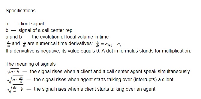
Deep neural networks for automatic call evaluation
Call evaluation is a key part of quality control for call centers. It allows organizations to fine-tune workflow so that operators can do work faster and more efficiently, as well as avoid meaningless routines.
Bearing in mind that the call center should be effective, we worked on automating the evaluation of calls. As a result, we came up with an algorithm that processes calls and distributes them into two groups: suspicious and neutral. All suspicious calls were immediately sent to the quality assessment team.

We took 1700 audio files for the samples and trained the network. Since the neuron initially did not know what was considered suspicious and neutral, we manually marked all the files accordingly.
')
In neutral samples, the operators are:
In suspicious patterns, operators often did the following:
When the algorithm finished processing the files, it marked 200 files as invalid. These files contained neither suspicious nor neutral signs. We found out what was in these 200 files:
When we deleted these files, we divided the remaining 1500 into training and test examples. Later we used these datasets to train and test the deep neural network.
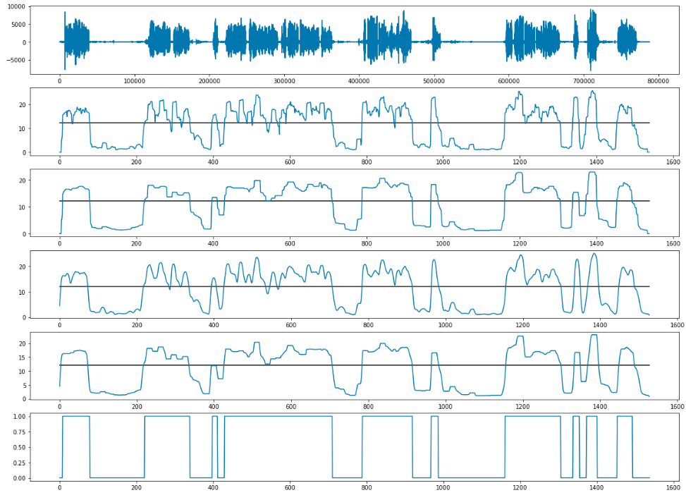
High-level feature extraction plays an important role in machine learning, since it directly affects the efficiency of the algorithm. After analyzing all possible sources, we selected the following signs:
Cepstral tone frequency coefficients and saturation vector are sensitive to the length of the input signal. We could extract them from the whole file at a time, but by doing so, we would have missed the development of the feature over time. Since this method did not suit us, we decided to divide the signal into “windows” (temporary blocks).
In order to improve the quality of the trait, we broke the signal into chunks, which partially overlapped each other. Next, we extracted the tag sequentially for each chunk; therefore, the attribute matrix was calculated for each audio file.
Window size - 0.2 s; window pitch - 0.1 s.
Our first approach to solving the problem is to define and process each phrase in the stream separately.
First of all, we did diarization and isolated all the phrases using the LIUM library. The input files were of poor quality, so at the output we also applied anti-aliasing and adaptive thresholding for each file.
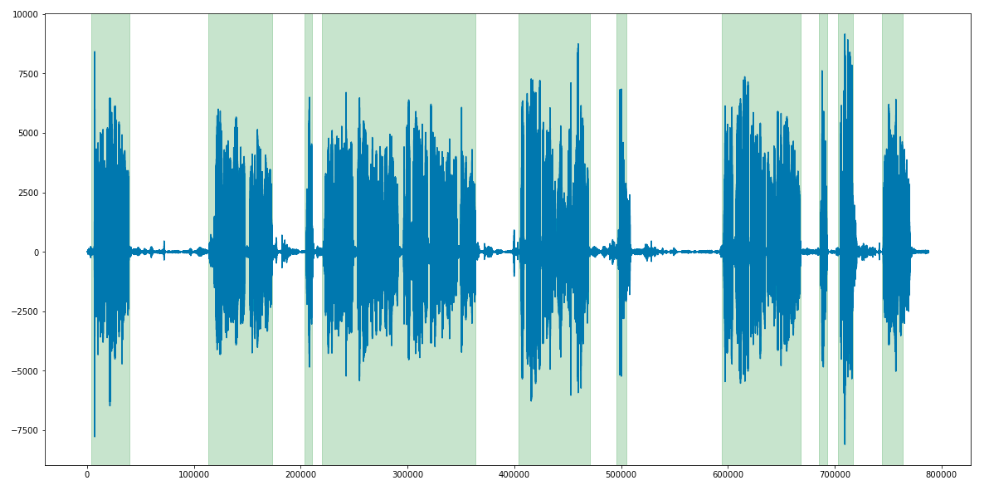
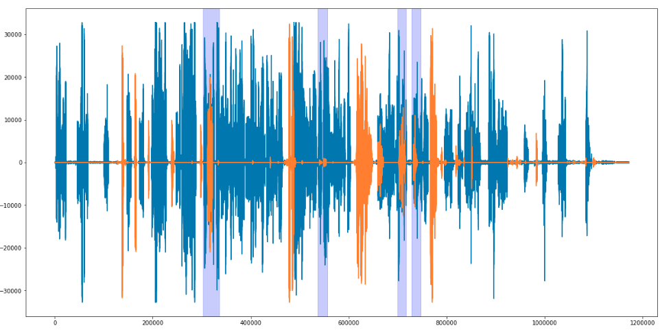
When we determined the time limits for each phrase (both client and operator), we imposed them on each other and found cases when both people speak at the same time, as well as cases when both are silent. It remained only to determine the magnitude of the threshold. We agreed that if 3 or more seconds are spoken to by the participants at the same time, this is considered interrupting. For silence, the threshold was set at 3 seconds smoothly.

The point is that each phrase has its own length. Therefore, the number of features extracted from each phrase is different.
The LSTM neural network could handle this problem. Networks of this kind can not only process sequences of different lengths, but they can also contain feedback, which gives you the opportunity to save information. These features are very important because the phrases spoken earlier contain information that affects the phrases said after.

Then we trained our LSTM network to determine the intonation of each phrase.
As a training set, we took 70 files with 30 phrases on average (15 phrases for each side).
The main goal was to evaluate the phrases of the call center operator, so we did not use client speech for training. We used 750 phrases as a training dataset, and 250 phrases as a test. As a result, Neuronka learned to classify speech with an accuracy of 72%.
But in the end, we were not satisfied with the performance of the LSTM network: working with it took too much time, and the results were far from perfect. Therefore, it was decided to use a different approach.
It is time to tell how we determined the tone of voice using XGBoost plus a combination of LSTM and XGB.
We marked files as suspicious if they contained at least one phrase that violated the rules. So we tagged 2500 files.
To extract features, we used the same method and the same ANN architecture, but with one difference: we scaled the architecture to fit the new dimensions of the features.
With optimal parameters, the neural network produced 85% accuracy.

The XGBoost model requires a fixed number of attributes for each file. To satisfy this requirement, we have created several signals and parameters.

The following statistics were used:
All indicators were calculated separately for each signal. The total number of signs is 36, with the exception of the record length. As a result, we had 37 numeric characters for each record.
The prediction accuracy of this algorithm is 0.869.
To combine classifiers, we crossed these two models. At the exit, this increased accuracy by 2%.

That is, we managed to improve the prediction accuracy to 0.9 ROC - AUC (Area Under Curve).
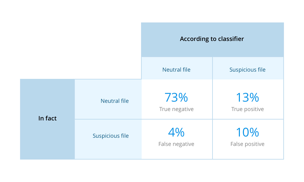
We tested our deep neural network on 205 files (177 neutral, 28 suspicious). The network had to process each file and decide which group it belongs to. Below are the results:
To estimate the percentage of correct / false results, we used the Error Matrix in the form of a 2x2 table.
We could not wait to try this approach to recognize words and phrases in audio files. The goal was to find files in which the call center operator was not presented to clients in the first 10 seconds of the conversation.
We took 200 phrases with an average length of 1.5 seconds, in which operators give their name and company name.
The search for such files manually took a lot of time, because I had to listen to each file in order to check if the necessary phrases were in it. To speed up the subsequent learning, we artificially increased the dataset: we changed each file randomly 6 times - added noise, changed the frequency and / or volume. So we got in 1500 files.
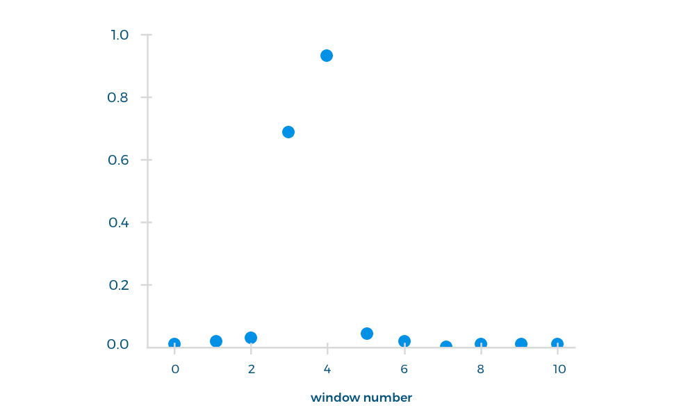
We used the first 10 seconds of the operator's response to train the classifier, because it was in this interval that the necessary phrase was uttered. Each such fragment was divided into windows (window length - 1.5 s, window pitch - 1 s) and processed by the neural network as an input file. As an output file, we obtained the probability of pronouncing each phrase in the selected window.
We drove another 300 files through the network to find out if the necessary phrase was uttered in the first 10 seconds. For these files, the accuracy was 87%.
Automatic call evaluation helps define clear KPIs for call center operators, highlight and follow best practices, and increase call center productivity. But It is worth noting that speech recognition software can also be used for a wider range of tasks.
Below are a few examples of how speech recognition can help organizations:
Bearing in mind that the call center should be effective, we worked on automating the evaluation of calls. As a result, we came up with an algorithm that processes calls and distributes them into two groups: suspicious and neutral. All suspicious calls were immediately sent to the quality assessment team.
How we trained deep neural network
We took 1700 audio files for the samples and trained the network. Since the neuron initially did not know what was considered suspicious and neutral, we manually marked all the files accordingly.
')
In neutral samples, the operators are:
- did not raise his voice;
- give customers all the requested information;
- did not respond to provocations from the client.
In suspicious patterns, operators often did the following:
- used obscene language;
- raised their voice or shouted at customers;
- passed on personalities;
- refused to advise on issues.
When the algorithm finished processing the files, it marked 200 files as invalid. These files contained neither suspicious nor neutral signs. We found out what was in these 200 files:
- the customer hung up immediately after the operator answered;
- the client said nothing after being answered;
- there was too much noise on the client or operator side.
When we deleted these files, we divided the remaining 1500 into training and test examples. Later we used these datasets to train and test the deep neural network.
Step 1: Extraction of the signs
High-level feature extraction plays an important role in machine learning, since it directly affects the efficiency of the algorithm. After analyzing all possible sources, we selected the following signs:
Time statistics
- Zero-crossing rate : the rate at which the signal changes from plus to negative and vice versa.
- The median frame energy is the sum of the signals squared and normalized by the corresponding frame length.
- Subframe energy entropy : entropy of the normalized energy of subframes. It can be interpreted as a measure of drastic changes.
- Mean / median / standard deviation of the frame .
Spectral statistics (with frequency intervals)
- Spectral centroid.
- Spectral distribution.
- Spectral entropy.
- Spectral radiation.
- Spectral attenuation.
Cepstral tone frequency coefficients and saturation vector are sensitive to the length of the input signal. We could extract them from the whole file at a time, but by doing so, we would have missed the development of the feature over time. Since this method did not suit us, we decided to divide the signal into “windows” (temporary blocks).
In order to improve the quality of the trait, we broke the signal into chunks, which partially overlapped each other. Next, we extracted the tag sequentially for each chunk; therefore, the attribute matrix was calculated for each audio file.
Window size - 0.2 s; window pitch - 0.1 s.
Step 2: we determine the tone of the voice in separate phrases
Our first approach to solving the problem is to define and process each phrase in the stream separately.
First of all, we did diarization and isolated all the phrases using the LIUM library. The input files were of poor quality, so at the output we also applied anti-aliasing and adaptive thresholding for each file.
Handling of interruptions and long silence
When we determined the time limits for each phrase (both client and operator), we imposed them on each other and found cases when both people speak at the same time, as well as cases when both are silent. It remained only to determine the magnitude of the threshold. We agreed that if 3 or more seconds are spoken to by the participants at the same time, this is considered interrupting. For silence, the threshold was set at 3 seconds smoothly.
The point is that each phrase has its own length. Therefore, the number of features extracted from each phrase is different.
The LSTM neural network could handle this problem. Networks of this kind can not only process sequences of different lengths, but they can also contain feedback, which gives you the opportunity to save information. These features are very important because the phrases spoken earlier contain information that affects the phrases said after.
Then we trained our LSTM network to determine the intonation of each phrase.
As a training set, we took 70 files with 30 phrases on average (15 phrases for each side).
The main goal was to evaluate the phrases of the call center operator, so we did not use client speech for training. We used 750 phrases as a training dataset, and 250 phrases as a test. As a result, Neuronka learned to classify speech with an accuracy of 72%.
But in the end, we were not satisfied with the performance of the LSTM network: working with it took too much time, and the results were far from perfect. Therefore, it was decided to use a different approach.
It is time to tell how we determined the tone of voice using XGBoost plus a combination of LSTM and XGB.
Determine the tone of voice for the entire file.
We marked files as suspicious if they contained at least one phrase that violated the rules. So we tagged 2500 files.
To extract features, we used the same method and the same ANN architecture, but with one difference: we scaled the architecture to fit the new dimensions of the features.
With optimal parameters, the neural network produced 85% accuracy.
Xgboost
The XGBoost model requires a fixed number of attributes for each file. To satisfy this requirement, we have created several signals and parameters.
The following statistics were used:
- The average value of the signal.
- The average value of the first 10 seconds of the signal.
- The average value of the last 3 seconds of the signal.
- The average value of local maxima in the signal.
- The average value of local maxima in the first 10 seconds of the signal.
- The average value of local maxima in the last 3 seconds of the signal.
All indicators were calculated separately for each signal. The total number of signs is 36, with the exception of the record length. As a result, we had 37 numeric characters for each record.
The prediction accuracy of this algorithm is 0.869.
LSTM and XGB combination
To combine classifiers, we crossed these two models. At the exit, this increased accuracy by 2%.
That is, we managed to improve the prediction accuracy to 0.9 ROC - AUC (Area Under Curve).
Result
We tested our deep neural network on 205 files (177 neutral, 28 suspicious). The network had to process each file and decide which group it belongs to. Below are the results:
- 170 neutral files were defined correctly;
- 7 neutral files were identified as suspicious;
- 13 suspicious files were identified correctly;
- 15 suspicious files were identified as neutral.
To estimate the percentage of correct / false results, we used the Error Matrix in the form of a 2x2 table.
Find a specific phrase in the conversation
We could not wait to try this approach to recognize words and phrases in audio files. The goal was to find files in which the call center operator was not presented to clients in the first 10 seconds of the conversation.
We took 200 phrases with an average length of 1.5 seconds, in which operators give their name and company name.
The search for such files manually took a lot of time, because I had to listen to each file in order to check if the necessary phrases were in it. To speed up the subsequent learning, we artificially increased the dataset: we changed each file randomly 6 times - added noise, changed the frequency and / or volume. So we got in 1500 files.
Total
We used the first 10 seconds of the operator's response to train the classifier, because it was in this interval that the necessary phrase was uttered. Each such fragment was divided into windows (window length - 1.5 s, window pitch - 1 s) and processed by the neural network as an input file. As an output file, we obtained the probability of pronouncing each phrase in the selected window.
We drove another 300 files through the network to find out if the necessary phrase was uttered in the first 10 seconds. For these files, the accuracy was 87%.
Actually, what is all this for?
Automatic call evaluation helps define clear KPIs for call center operators, highlight and follow best practices, and increase call center productivity. But It is worth noting that speech recognition software can also be used for a wider range of tasks.
Below are a few examples of how speech recognition can help organizations:
- collect and analyze data to improve voice UX;
- analyze call records to identify connections and trends;
- recognize people by voice;
- find and define customer emotions to improve user satisfaction;
- increase the average revenue per call;
- reduce the outflow;
- and much more!
Source: https://habr.com/ru/post/428598/
All Articles