We approximate the function using a neural network

In order to master libraries for working with neural networks, we will solve the problem of approximating the function of a single argument using neural network algorithms for learning and prediction.

Introduction

Let the function f: [x0, x1] -> R be given

We approximate the given function f by the formula

P(x) = SUM W[i]*E(x,M[i]) 

Where

• i = 1..n
• M [i] of R
• W [i] of R
• E (x, M) = {0, with x <M; 1/2, with x = M; 1, with x> M

Obviously, with a uniform distribution of the values ​​of M [i] on the segment (x0, x1), there are values ​​W [i] for which the formula P (x) would best approximate the function f (x). In this case, for given values ​​of M [i], defined on the interval (x0, x1) and ordered in increasing order, one can describe a sequential algorithm for calculating the values ​​of W [i] for the formula P (x).

And here is the neural network

We transform the formula P (x) = SUM W [i] * E (x, M [i]) to a neural network model with one input neuron, one output neuron, and n neurons of the hidden layer

 P(x) = SUM W[i]*S(K[i]*x + B[i]) + C 

Where

• variable x - "input" layer consisting of one neuron
• {K, B} - parameters of the "hidden" layer, consisting of n neurons and the activation function - sigmoid
• {W, C} - the parameters of the "output" layer, consisting of one neuron, which calculates the weighted sum of its inputs.
• S - sigmoid,

wherein

• initial parameters of the "hidden" layer K [i] = 1
• the initial parameters of the "hidden" layer B [i] are uniformly distributed on the segment (-x1, -x0)

All parameters of the neural network K, B, W and C are determined by training the neural network on samples (x, y) of the values ​​of the function f.

Sigmoid

Sigmoid is a smooth monotone increasing non-linear function.

• S (x) = 1 / (1 + exp (-x)).

Program

We use Tensorflow package to describe our neural network.

 #        x = tf.placeholder(tf.float32, [None, 1], name="x") #        y = tf.placeholder(tf.float32, [None, 1], name="y") #   nn = tf.layers.dense(x, hiddenSize, activation=tf.nn.sigmoid, kernel_initializer=tf.initializers.ones(), bias_initializer=tf.initializers.random_uniform(minval=-x1, maxval=-x0), name="hidden") #   model = tf.layers.dense(nn, 1, activation=None, name="output") #    cost = tf.losses.mean_squared_error(y, model) train = tf.train.GradientDescentOptimizer(learn_rate).minimize(cost) 

Training

 init = tf.initializers.global_variables() with tf.Session() as session: session.run(init) for _ in range(iterations): train_dataset, train_values = generate_test_values() session.run(train, feed_dict={ x: train_dataset, y: train_values }) 

Full text

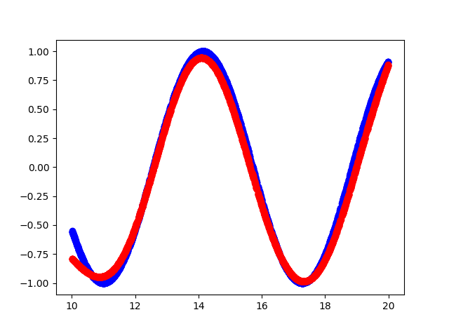
 import math import numpy as np import tensorflow as tf import matplotlib.pyplot as plt x0, x1 = 10, 20 #    test_data_size = 2000 #      iterations = 20000 #    learn_rate = 0.01 #   hiddenSize = 10 #    #     def generate_test_values(): train_x = [] train_y = [] for _ in range(test_data_size): x = x0+(x1-x0)*np.random.rand() y = math.sin(x) #   train_x.append([x]) train_y.append([y]) return np.array(train_x), np.array(train_y) #        x = tf.placeholder(tf.float32, [None, 1], name="x") #        y = tf.placeholder(tf.float32, [None, 1], name="y") #   nn = tf.layers.dense(x, hiddenSize, activation=tf.nn.sigmoid, kernel_initializer=tf.initializers.ones(), bias_initializer=tf.initializers.random_uniform(minval=-x1, maxval=-x0), name="hidden") #   model = tf.layers.dense(nn, 1, activation=None, name="output") #    cost = tf.losses.mean_squared_error(y, model) train = tf.train.GradientDescentOptimizer(learn_rate).minimize(cost) init = tf.initializers.global_variables() with tf.Session() as session: session.run(init) for _ in range(iterations): train_dataset, train_values = generate_test_values() session.run(train, feed_dict={ x: train_dataset, y: train_values }) if(_ % 1000 == 999): print("cost = {}".format(session.run(cost, feed_dict={ x: train_dataset, y: train_values }))) train_dataset, train_values = generate_test_values() train_values1 = session.run(model, feed_dict={ x: train_dataset, }) plt.plot(train_dataset, train_values, "bo", train_dataset, train_values1, "ro") plt.show() with tf.variable_scope("hidden", reuse=True): w = tf.get_variable("kernel") b = tf.get_variable("bias") print("hidden:") print("kernel=", w.eval()) print("bias = ", b.eval()) with tf.variable_scope("output", reuse=True): w = tf.get_variable("kernel") b = tf.get_variable("bias") print("output:") print("kernel=", w.eval()) print("bias = ", b.eval()) 

That's what happened

• Blue color - the original function
• Red color - function approximation

Console output

 cost = 0.15786637365818024 cost = 0.10963975638151169 cost = 0.08536215126514435 cost = 0.06145831197500229 cost = 0.04406769573688507 cost = 0.03488277271389961 cost = 0.026663536205887794 cost = 0.021445846185088158 cost = 0.016708852723240852 cost = 0.012960446067154408 cost = 0.010525770485401154 cost = 0.008495906367897987 cost = 0.0067353141494095325 cost = 0.0057082874700427055 cost = 0.004624188877642155 cost = 0.004093789495527744 cost = 0.0038146725855767727 cost = 0.018593043088912964 cost = 0.010414039716124535 cost = 0.004842184949666262 hidden: kernel= [[1.1523403 1.181032 1.1671464 0.9644377 0.8377886 1.0919508 0.87283015 1.0875995 0.9677301 0.6194152 ]] bias = [-14.812331 -12.219926 -12.067375 -14.872566 -10.633507 -14.014006 -13.379829 -20.508204 -14.923473 -19.354435] output: kernel= [[ 2.0069902 ] [-1.0321712 ] [-0.8878887 ] [-2.0531905 ] [ 1.4293027 ] [ 2.1250408 ] [-1.578137 ] [ 4.141281 ] [-2.1264815 ] [-0.60681605]] bias = [-0.2812019] 

Source

https://github.com/dprotopopov/nnfunc