How to interpret model predictions in SHAP
One of the most important tasks in the field of data science is not only building a model capable of making qualitative predictions, but also the ability to interpret such predictions.
If we do not just know that the customer is inclined to buy goods, but also understand what affects their purchase, we will be able to build a company strategy in the future, aimed at increasing sales efficiency.
Or the model predicted that the patient would soon get sick. The accuracy of such predictions is not very high, because there are many factors hidden from the model, but an explanation of the reasons why the model made such a prediction can help the doctor pay attention to new symptoms. Thus, it is possible to expand the boundaries of the model, if its accuracy itself is not too high.
In this post I want to talk about the technique of SHAP , which allows you to look under the hood of a variety of models.
')
If everything is more or less clear with linear models, the greater the absolute value of the coefficient under the predictor, the more important this predictor is, then the importance of features of the same gradient boosting is much more difficult to explain.

On the sklearn stack, in the xgboost, lightGBM packages, there were built-in methods of feature importance for “wooden models”:
The main problem in all these approaches is that it is not clear how this feature affects the prediction of the model. For example, we learned that the level of income is important for assessing the solvency of a bank’s customer to pay off a loan. But how exactly? How much higher income shifts model predictions?
Of course, we can make several predictions by changing the level of income. But what to do with other features? After all, we find ourselves in the situation that it is necessary to gain an understanding of the influence of income, independently of other features, with their average value.
There is a sort of average bank customer "in a vacuum." How will the predictions of the model change depending on the change in income?
This is where the SHAP library comes to the rescue.
In the SHAP library, to calculate the importance of features, Shapley values are calculated (after the name of the American mathematician and the library is named).
To assess the importance of the feature, the prediction of the model is evaluated with and without this feature.

Shapley values come from game theory.
Consider the scenario: a group of people playing cards. How to distribute the prize fund between them in accordance with their contribution?
A number of assumptions are made:
We present the features of the model as players, and the prize pool as the final prediction of the model.
The formula for calculating the Shaply value for the i-th feature:
Here:
- this is the prediction of the model with the i-th feature,
- this is a model prediction without an i-feature,
- number of features,
- arbitrary set of features without the i-th feature
The Shaply value for the i-th feature is calculated for each sample of data (for example, for each client in the sample) on all possible combinations of features (including the absence of all features), then the values obtained are summed modulo and the resulting importance of the i-th feature is obtained.
These calculations are extremely costly, so various algorithms for optimization of calculations are used under the hood, for more details, see the link above on the githabe.
Take the vanilla example from the xgboost documentation .
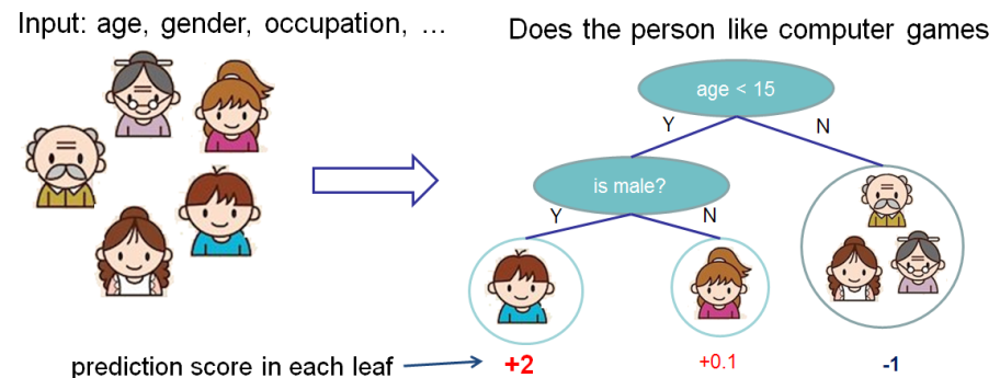
We want to appreciate the importance of features for predicting whether a person likes computer games.
In this example, for simplicity, we have two features: age (age) and gender (gender). Gender (floor) takes values 0 and 1.
Take Bobby (the little boy in the leftmost node of the tree) and calculate the Shaply value for the age feature.
We have two sets of features S:
- no features,
- there is only a feature floor.
Different models work differently with situations when there are no features for sample data, that is, for all features, the values are NULL.
It will be considered in this case that the model averages the predictions by the branches of the tree, that is, the prediction without features will be .
If we add age knowledge, the prediction of the model will be .
As a result, the value of Shaply for the case of the absence of features:
For bobby for prediction without features age, only with features gender . If we know age, then prediction is the leftmost tree, that is, 2.
As a result, the Shaply value for this case:
Total Shaply value for feature age (age):
The SHAP library has a rich visualization functionality that helps to easily and simply explain the model for both the business and the analyst himself in order to assess the adequacy of the model.
On one of the projects, I analyzed the outflow of employees from the company. Xgboost was used as a model.
Code in python:
The resulting graph of the importance of features:
How to read it:
From the graph you can draw interesting conclusions and check their adequacy:
You can immediately form a portrait of the outgoing employee: he did not get a salary, he is young enough, single for a long time in one position, there was no grade increase, there were no high annual assessments, he began to communicate with his colleagues a little.
Simple and convenient!
You can explain the prediction for a particular employee:
Or see the dependence of predictions on a specific feature in the form of 2D graphics:
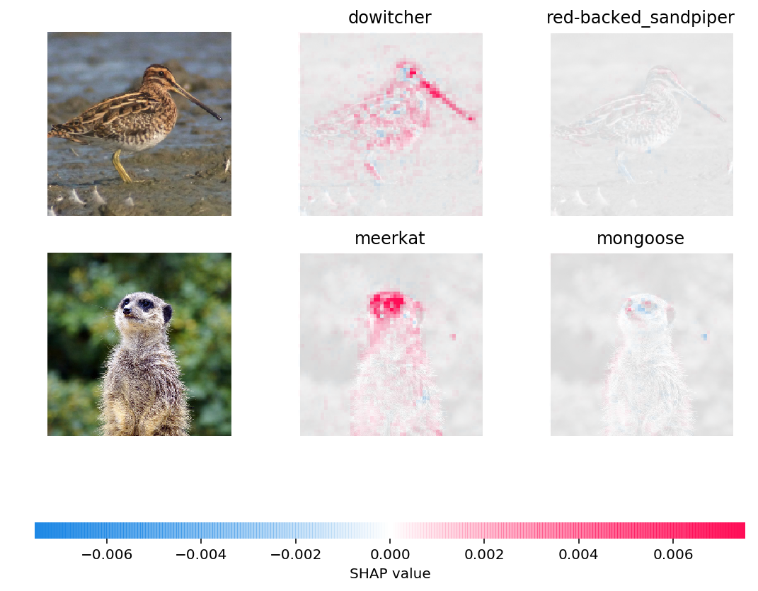
You can even visualize the predictions of neural networks in the pictures:
I myself learned about SHAP values about six months ago and this completely replaced other methods for assessing the importance of features.
Main advantages:
If we do not just know that the customer is inclined to buy goods, but also understand what affects their purchase, we will be able to build a company strategy in the future, aimed at increasing sales efficiency.
Or the model predicted that the patient would soon get sick. The accuracy of such predictions is not very high, because there are many factors hidden from the model, but an explanation of the reasons why the model made such a prediction can help the doctor pay attention to new symptoms. Thus, it is possible to expand the boundaries of the model, if its accuracy itself is not too high.
In this post I want to talk about the technique of SHAP , which allows you to look under the hood of a variety of models.
')
If everything is more or less clear with linear models, the greater the absolute value of the coefficient under the predictor, the more important this predictor is, then the importance of features of the same gradient boosting is much more difficult to explain.
Why there was a need for such a library
On the sklearn stack, in the xgboost, lightGBM packages, there were built-in methods of feature importance for “wooden models”:
- Gain
This measure shows the relative contribution of each feature to the model. for calculation, we go through each tree, look at each node of the tree, which feature leads to a node splitting and how much uncertainty of the model is reduced according to the metric (Gini impurity, information gain).
For each feature, its contribution is summed over all trees. - Cover
Shows the number of observations for each feature. For example, you have 4 features, 3 trees. Suppose feature 1 in the tree nodes contains 10, 5, and 2 observations in trees 1, 2, and 3, respectively. Then, for this feature, the importance will be 17 (10 + 5 + 2). - Frequency
It shows how often this feature is found in the tree nodes, that is, the total number of tree partitions into nodes for each feature in each tree is considered.
The main problem in all these approaches is that it is not clear how this feature affects the prediction of the model. For example, we learned that the level of income is important for assessing the solvency of a bank’s customer to pay off a loan. But how exactly? How much higher income shifts model predictions?
Of course, we can make several predictions by changing the level of income. But what to do with other features? After all, we find ourselves in the situation that it is necessary to gain an understanding of the influence of income, independently of other features, with their average value.
There is a sort of average bank customer "in a vacuum." How will the predictions of the model change depending on the change in income?
This is where the SHAP library comes to the rescue.
Calculate the importance of features using SHAP
In the SHAP library, to calculate the importance of features, Shapley values are calculated (after the name of the American mathematician and the library is named).
To assess the importance of the feature, the prediction of the model is evaluated with and without this feature.
A bit of prehistory
Shapley values come from game theory.
Consider the scenario: a group of people playing cards. How to distribute the prize fund between them in accordance with their contribution?
A number of assumptions are made:
- The amount of remuneration of each player is equal to the total amount of the prize fund.
- If two players have made an equal contribution to the game, they will receive an equal reward.
- If the player has made no contribution, he does not receive a reward.
- If a player has spent two games, then his total remuneration consists of the amount of rewards for each of the games.
We present the features of the model as players, and the prize pool as the final prediction of the model.
Consider an example
The formula for calculating the Shaply value for the i-th feature:
$$ display $$ \ begin {equation *} \ phi_ {i} (p) = \ sum_ {S \ subseteq N / \ {i \}} \ frac {| S |! (n - | S | -1) !} {n!} (p (S \ cup \ {i \}) - p (S)) \ end {equation *} $$ display $$
Here:
- this is the prediction of the model with the i-th feature,
- this is a model prediction without an i-feature,
- number of features,
- arbitrary set of features without the i-th feature
The Shaply value for the i-th feature is calculated for each sample of data (for example, for each client in the sample) on all possible combinations of features (including the absence of all features), then the values obtained are summed modulo and the resulting importance of the i-th feature is obtained.
These calculations are extremely costly, so various algorithms for optimization of calculations are used under the hood, for more details, see the link above on the githabe.
Take the vanilla example from the xgboost documentation .
We want to appreciate the importance of features for predicting whether a person likes computer games.
In this example, for simplicity, we have two features: age (age) and gender (gender). Gender (floor) takes values 0 and 1.
Take Bobby (the little boy in the leftmost node of the tree) and calculate the Shaply value for the age feature.
We have two sets of features S:
- no features,
- there is only a feature floor.
Situation when there are no feature values
Different models work differently with situations when there are no features for sample data, that is, for all features, the values are NULL.
It will be considered in this case that the model averages the predictions by the branches of the tree, that is, the prediction without features will be .
If we add age knowledge, the prediction of the model will be .
As a result, the value of Shaply for the case of the absence of features:
The situation when we know the floor
For bobby for prediction without features age, only with features gender . If we know age, then prediction is the leftmost tree, that is, 2.
As a result, the Shaply value for this case:
$$ display $$ \ begin {equation *} \ frac {| S |! (n - | S | -1)!} {n!} (p (S \ cup \ {i \}) - p (S) ) = \ frac {1 (2-1-1)!} {2!} (1.975) = 0.9875 \ end {equation *} $$ display $$
Summarize
Total Shaply value for feature age (age):
$$ display $$ \ begin {equation *} \ phi_ {Age Bobby} = 0.9875 + 0.5125 = 1.5 \ end {equation *} $$ display $$
Real example from business
The SHAP library has a rich visualization functionality that helps to easily and simply explain the model for both the business and the analyst himself in order to assess the adequacy of the model.
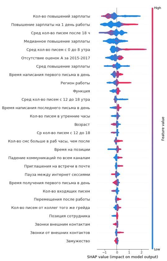
On one of the projects, I analyzed the outflow of employees from the company. Xgboost was used as a model.
Code in python:
import shap shap_test = shap.TreeExplainer(best_model).shap_values(df) shap.summary_plot(shap_test, df, max_display=25, auto_size_plot=True) The resulting graph of the importance of features:
How to read it:
- the values to the left of the central vertical line are negative class (0), to the right positive (1)
- the thicker the line on the graph, the more such observation points
- the redder the point on the graph, the higher the feature values in it
From the graph you can draw interesting conclusions and check their adequacy:
- the less an employee is paid a salary, the higher the likelihood of his leaving
- There are regions of offices, where the outflow is higher
- the younger the employee, the higher the likelihood of his leaving
- ...
You can immediately form a portrait of the outgoing employee: he did not get a salary, he is young enough, single for a long time in one position, there was no grade increase, there were no high annual assessments, he began to communicate with his colleagues a little.
Simple and convenient!
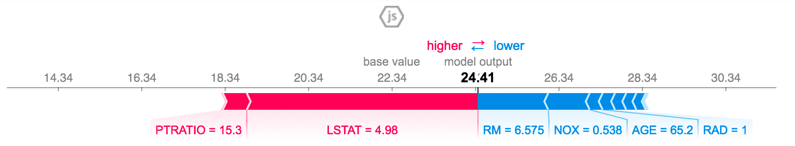
You can explain the prediction for a particular employee:
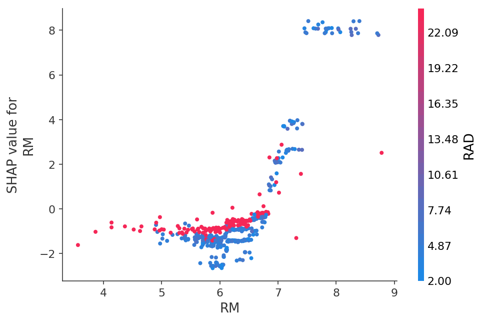
Or see the dependence of predictions on a specific feature in the form of 2D graphics:
You can even visualize the predictions of neural networks in the pictures:
Conclusion
I myself learned about SHAP values about six months ago and this completely replaced other methods for assessing the importance of features.
Main advantages:
- convenient visualization and interpretation
- honest calculation of the importance of features
- the ability to evaluate features for a specific subsample of data (for example, how our customers differ from other clients in the sample) is done with a simple dataset filter in pandas and its analysis in the shap, literally a couple of lines of code
Source: https://habr.com/ru/post/428213/
All Articles