Implementation of the Levenberg-Marquardt algorithm for optimizing neural networks on TensorFlow

This is a tensial for the TensorFlow library. Consider it a little deeper than in the articles about the recognition of handwritten numbers. This is a tutorial on optimization techniques. Quite without mathematics is not enough. It's okay if you completely forget it. Recall. There will be no formal evidence and complex conclusions, only the necessary minimum for an intuitive understanding. For a start, a little background on how this algorithm can be useful in optimizing a neural network.

Six months ago, a friend asked me to show how to make a neural network in Python. His company produces instruments for geophysical measurements. Several different probes measure the set of signals associated with the parameters of the surrounding environment during the drilling process. In some difficult cases, the parameters of the medium can be accurately calculated from the signals for a long time even on a powerful computer, and it is necessary to interpret the results of measurements in the field. There was an idea to count several hundred thousand cases on a cluster, and to train a neural network on them. Since the neural network works very quickly, it can be used to determine parameters that are consistent with the measured signals, right during the drilling process. Details are in the article:

Kushnir, D., Velker, N., Bondarenko, A., Dyatlov, G., & Dashevsky, Y. (2018, October 29). Real-Time Simulation of the 2D Azimuthal Resistivity Resistance Tool for 2D Fault Model Using Neural Networks (Russian). Society of Petroleum Engineers. doi: 10.2118 / 192573-RU

One evening I showed how keras implement a simple neural network, and a friend at work started training on counted data. A couple of days discussed the result. From my point of view, he looked promising, but a friend said that he needed calculations with the accuracy of the instrument. And if the mean square error ( mean squared error ) turned out to be in area 1, then 1e-3 was needed. 3 orders less. A thousand times.

Experiments with the neural network architecture, data normalization, optimization approaches yielded almost nothing. A couple of weeks a friend called and said that he installed MatLab and solved the problem using the Levenberg-Marquardt method (hereinafter we will call LM ). It was optimized for a long time (several days), did not work on the GPU, but the result was correct. It sounded like a challenge.

A quick search for a ready-made LM optimizer for keras or TensorFlow did not work. I came across only the pyrenn library, but its functionality seemed poor to me. Decided to implement independently. At first glance, everything looked simple, and two evenings should have been enough. Carried longer. There were two problems:

TensorFlow. A lot of articles, but almost all of the level "but let's write ~~hello world~~ handwritten digits recognition."
Maths. I have forgotten a lot, but the authors of mathematical articles do not care at all about people like me: solid formulas without explanations, “obvious!” And so on.

As a result, I wrote an article for those who have forgotten math and want to understand TensorFlow a little deeper, but without hardcore. The article has a lot of text and little code. The reverse option, when there is little text and a lot of code, is here Jupyter Notebook Levenberg-Marquardt .

Get to know Rosenbrock's function

The training data will be generated by the Rosenbrock function , which is often used as a reference test of optimization algorithms:

$f (x, y) = (a-x) ^ 2 + b (y-x ^ 2) ^ 2$

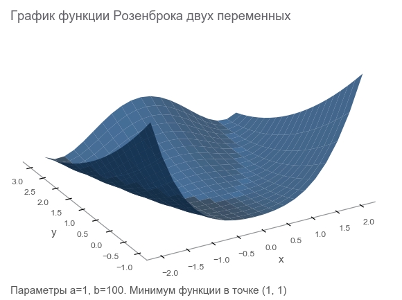
What is she good at?

Beautiful schedule. Rosenbrock 's banana function is called Rosenbrock valley and untranslatable.
The global minimum is inside a long, narrow, parabolic flat valley. Finding a valley is trivial, and a global minimum is difficult.
There is a multi-dimensional option. To come up with a good function of many variables is not so simple.

We will start writing code with it by connecting the necessary libraries for further work:

import numpy as np import tensorflow as tf import math def rosenbrock(x, y, a, b): return (a - x)**2 + b*(y - x**2)**2

We formulate the problem

Since we were talking about a measuring device, let's continue using the analogy. Our device in the fictional world can measure coordinates $(x, y)$ and height $z$ . Physicists studied the world and said: " Yes, it's Rosenbrock! Knowing the coordinates, you can accurately calculate the height, you do not need to measure it. " In other words, scientists gave us a model. $z = rosenbrock (x, y, a, b)$ which depends on the parameters $(a, b)$ . These parameters, though constant in the fictional world, are unknown. They need to find.

We conducted a series of experiments that gave $m$ points $(x_1, y_1, z_1), (x_2, y_2, z_2), ..., (x_m, y_m, z_m)$ :

 # (2.5, 2.5) -   ,  ,     data_points = np.array([[x, y, rosenbrock(x, y, 2.5, 2.5)] for x in np.arange(-2, 2.1, 2) for y in np.arange(-2, 2.1, 2)]) m = data_points.shape[0]

The first way to optimize is to try to guess the parameters. Let's use the Numpy library:

 x, y = data_points[:, 0], data_points[:, 1] z = data_points[:, 2] #   =5  b=5? a_guess, b_guess = 5., 5. #  -hat   ,   , #   ,   ,   .   #     ^   - # .    hat. z_hat = rosenbrock(x, y, a_guess, b_guess)

How to understand how wrong we are? Calculate residuals - the size of the errors. $m$ points give $m$ residuals - need an integral indicator. Let us square each residual and calculate the average:

$MSE (a, b) = \ frac {1} {m} \ sum_ {i = 1} ^ {m} (z_ {i} - \ widehat {z_ {i}}) ^ 2$

Such a measure of proximity is called the mean square error ( mean squared error , hereinafter referred to as mse ):

 # r - residuals () r = z - z_hat # mse loss = np.mean(r**2) print(loss)

 [Out]: 3868.2291666666665

Minimizing mse , we solve the problem of least squares ( nonlinear squares minimization ):

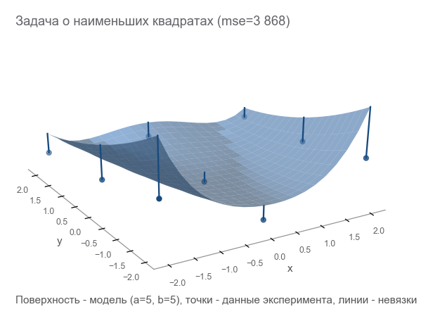
It is seen that the parameters did not guess at all.

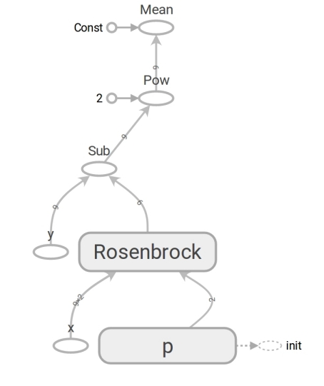
We formulate the problem on TensorFlow

The model has the form $z = rosenbrock (x, y, a, b)$ . We bring it to mind $y = f (x, p)$ (usually mathematicians write $\ beta$ instead $p$ , but programmers do not use beta). Now the model has the form $y = rosenbrock (x, p)$ where $y$ - height, $x$ - the vector of coordinates of two elements (components), and $p$ - vector of parameters.

Programmers often think of vectors as one-dimensional arrays. This is not entirely correct. An array of numbers is a means of representing a vector. You can represent a vector by an array of dimension $N$ two-dimensional array $1 \ times N$ and even an array $N \ times 1$ in cases when the fact that the vector is a column vector is important (for example, to multiply the matrix by it):

$\ begin {bmatrix} x_1 \\\ vdots \\ x_N \ end {bmatrix}$

TensorFlow uses the notion of tensor . A tensor , like an array, can be one-dimensional (to represent a vector ), two-dimensional (for a matrix or a column vector ), and any higher dimension.

 #    ('placeholder' ,    #      ) x = tf.placeholder(tf.float64, shape=[m, 2]) y = tf.placeholder(tf.float64, shape=[m]) #   ('variable' ,    ) #     (5, 5) p = tf.Variable([5., 5.], dtype=tf.float64) #  y_hat = rosenbrock(x[:, 0], x[:, 1], p[0], p[1]) #  r = y - y_hat # mse (mean squared error) loss = tf.reduce_mean(r**2)

The code on TensorFlow does not differ in form from the code on Numpy. The content is huge. The Numpy code calculates the mse value . The code on TensorFlow does not perform any calculations at all; it forms a dataflow graph ( dataflow graph ) that can calculate mse. A very enduring brain is the work of the rosenbrock function. We use it in both cases. But when we pass Numpy arrays, it performs calculations using the formula and returns numbers. And when we transfer tensors TensorFlow, it forms a subgraph of the data stream and returns its edge ( edge ) in the form of a tensor. The wonders of polymorphism, but do not abuse them:

Due to the presence of such a data flow graph, TensorFlow, in particular, is able to calculate derivatives automatically (using reverse mode automatic differentiation ).

Minute math. Blocks "for those who have forgotten" will be hidden in the spoiler.

Derivative (number entered - number left)

Most likely you remember the definition of the derivative of a scalar (number-returning) function of one variable: for $f: \ mathbb {R} \ rightarrow \ mathbb {R}$ , derivative $f$ at the point $x \ in \ mathbb {R}$ is defined as:

${f} '(x) = \ lim_ {h \ to 0} \ frac {f (x + h) -f (x)} {h}$

Derivatives are a way to measure change . In the scalar case, the derivative shows how much the function changes. $f$ , if a $x$ will change to a small value $\ varepsilon$ :

$f (x + \ varepsilon) \ approx f (x) + \ varepsilon {f} '(x)$

For convenience, we further denote $y = f (x)$ and derivative $y$ by $x$ we write as $\ frac {\ partial y} {\ partial x}$ . Such a record emphasizes that $\ frac {\ partial y} {\ partial x}$ - the rate of change between variables $x$ and $y$ . More specifically, if $x$ will change to $\ varepsilon$ then $y$ will change by about $\ varepsilon \ frac {\ partial y} {\ partial x}$ . You can also write it like this:

$x \ rightarrow x + \ Delta x \ Rightarrow y \ rightarrow \ approx y + \ frac {\ partial y} {\ partial x} \ Delta x$

Reads like: "changing $x$ on $x + \ Delta x$ we change $y$ at about $y + \ Delta x \ frac {\ partial y} {\ partial x}$ ". Such a record clearly emphasizes the connection between the change $x$ and change $y$ .

We built the data flow graph, let's run the mse calculation:

 #        #      placeholder (  ) feed_dict = {x: data_points[:,0:2], y: data_points[:,2]} #       TensorFlow session = tf.Session() #     session.run(tf.global_variables_initializer()) #   ()  loss (mse) current_loss = session.run(loss, feed_dict) print(current_loss)

 [Out]: 3868.2291666666665

It turned out the same result as with the Numpy. So they were not mistaken.

Let's start optimizing

Unfortunately, the parameters could not be guessed. But then we:

Set the optimality criterion - the minimum value of mse.
Identified variable parameters: vector $p$ with components $a$ , $b$ Rosenbrock functions.
While not thinking about the restrictions, but they are not.

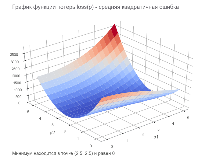
At the last step, we constructed a data flow graph with a finite loss tensor ( loss function ). The goal of optimization is to find the value of the parameter vector. $p$ at which the value of the loss function is minimal. We were lucky, the graph of this function is very simple (concave and without local minima):

Getting to the optimization. First, let's write a generic loop:

 # :   mse,   ,  #   mse,        placeholder def train(target_loss, max_steps, loss_tensor, train_step_op, inputs): step = 0 current_loss = session.run(loss_tensor, inputs) #           while current_loss > target_loss and step < max_steps: step += 1 #    1, 2, 4, 8, 16...  if math.log(step, 2).is_integer(): print(f'step: {step}, current loss: {current_loss}') #    session.run(train_step_op, inputs) current_loss = session.run(loss_tensor, inputs) print(f'ENDED ON STEP: {step}, FINAL LOSS: {current_loss}')

Optimize with the fastest gradient descent method (SGD)

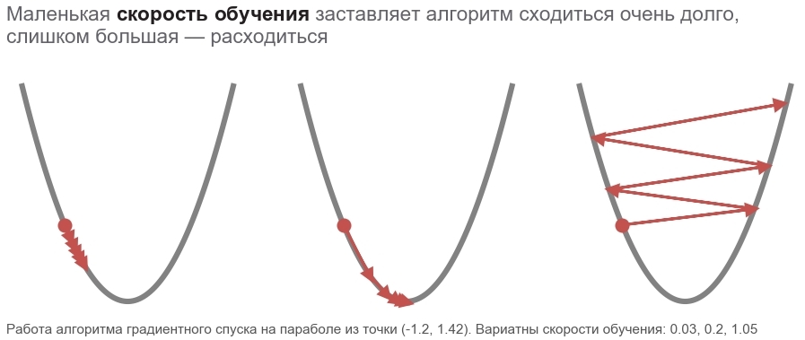
The actions of this method can be compared with the ride of a daring skier who always puts skis along the line of a falling slope (in the steepest direction down). This takes into account only the slope at the point of location. And if the slope is strong, then the skier flies a long distance until the next conversion. With a weak bias, it moves in small steps. Maybe how to fly away ~~into a tree~~ (the algorithm diverges ), and get stuck in the pit ( local minimum ).

You can record this way (we change $\ boldsymbol {p}$ on $\ boldsymbol {p} - ...$ ):

$\ boldsymbol {p} \ rightarrow \ boldsymbol {p} - \ alpha [\ nabla_ {p} loss (\ boldsymbol {p})]$

Fatty $\ boldsymbol {p}$ emphasizes that this is the point of the actual location - the value of the vector of parameters in the current step. In the first step, this is our guess (5, 5). There are two interesting points in the formula: $\ alpha$ - learning rate ( learning rate ), $\ nabla_ {p} loss$ - gradient of the loss function for the vector of parameters.

Gradient (vector in - number out)

Consider a function that accepts a vector as input and gives a scalar: $f: \ mathbb {R} ^ {N} \ rightarrow \ mathbb {R}$ . Derivative $f$ at the point $x \ in \ mathbb {R} ^ {N}$ now called gradient and is a vector $[\ nabla_ {x} f (x)] \ in \ mathbb {R} ^ {N}$ (reads "nabla"), composed of partial derivatives ( partial derivatives ):

$\ nabla_ {x} y = (\ frac {\ partial y} {\ partial x_ {1}}, \ frac {\ partial y} {\ partial x_ {2}}, ..., \ frac {\ partial y} {\ partial x_ {N}})$

For this case, the record of the dependence of the change of the function on the change of the argument is as follows:

$x \ rightarrow x + \ Delta x \ Rightarrow y \ rightarrow \ approx y + \ nabla_ {x} y \ cdot \ Delta x$

The record has changed quite a bit to accommodate that $x$ , $\ Delta x$ and $\ nabla_ {x} y$ - vectors in $\ mathbb {R} ^ {N}$ , but $y$ - scalar. When multiplying vectors $\ nabla_ {x} y$ and $\ Delta x$ scalar product is used (the sum of the products of the components).

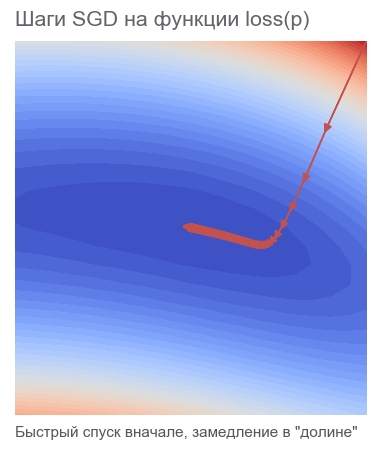
 #        grad = tf.gradients(loss, p)[0] #   learning_rate = 0.0005 #   ,     apply_gradients - #         opt = tf.train.GradientDescentOptimizer(learning_rate=1) #           sgd = opt.apply_gradients([(learning_rate*grad, p)]) #   ,    40000  session.run(tf.global_variables_initializer()) train(1e-10, 40000, loss, sgd, feed_dict) print('PARAMETERS:', session.run(p))

 [Out]: step: 1, current loss: 3868.2291666666665 step: 2, current loss: 1381.5379689135807 [...] ENDED ON STEP: 582, FINAL LOSS: 9.698531012270816e-11 PARAMETERS: [2.50000205 2.49999959]

It took 582 steps:

Movement towards antigradient

Why move in the opposite direction of the gradient? Recall the scalar product entry: $x \ rightarrow x + \ Delta x \ Rightarrow y \ rightarrow \ approx y + \ nabla_ {x} y \ cdot \ Delta x$ . Minimizing $y$ . Since the behavior of the function is known only in a small neighborhood through the derivative, it is necessary to move in small but optimal steps, minimizing the product $\ nabla_ {x} y \ cdot \ Delta x$ . According to the school definition, the scalar product of two vectors is a number equal to the product of the lengths of these vectors and the cosine of the angle between them : $a \ cdot b = \ left | a \ right | \ left | b \ right | cos \ angle (a, b)$ . For a fixed length of the vectors, this product reaches a minimum with a cosine of -1, i.e. at an angle of 180 degrees, when the vectors are directed in opposite directions. Accordingly, the minimum scalar product $\ nabla_ {x} y \ cdot \ Delta x$ achieved at $\ Delta x$ towards antigradient .

Optimize Adam Method

We will not further delve into the gradient methods, but there are lots of variations. You can read about them in the article Methods of optimization of neural networks . In TensorFlow, many optimizers are already implemented. For example, Adam:

 #       , #      adm = tf.train.AdamOptimizer(15).minimize(loss) #   ,    40000  session.run(tf.global_variables_initializer()) train(1e-10, 40000, loss, adm, feed_dict) print('PARAMETERS:', session.run(p))

 [Out]: step: 1, current loss: 3868.2291666666665 step: 2, current loss: 34205.72916492336 [...] ENDED ON STEP: 317, FINAL LOSS: 2.424142714263483e-12 PARAMETERS: [2.49999969 2.50000008]

Coped in 317 steps. Much faster.

We optimize by Newton's method

The actions of the second-order methods can be compared with the drive of a reasonable free-rider snowboarder, who thinks over the next point of his route for a long time and takes into account not only the bias at the point of location, but also the curvature.

In fact, both gradient descent methods and second-order methods try to guess ( approximate ) a function by the current point. Gradient methods are oriented only on the slope of the function graph at a point — the first derivative. The methods of the second order except for the slope take into account the curvature ( curvature ) - the second derivative: "if the curvature remains, where will be the minimum?". We calculate and go there:

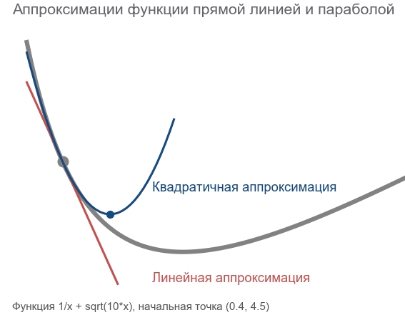
To build such an approximation and calculate the estimated minimum point, you can use the Taylor series ( Taylor series ). For the one-dimensional case, the approximation by a second-order polynomial at the point $a$ looks like that:

$f (x) \ approx f (a) + \ frac {f '(a) (x-a)} {1!} + \ frac {f' '(a) (x-a) ^ 2} {2!}$

The minimum is reached at $x = a - \ frac {f '(a)} {f' '(a)}$ . The multidimensional case looks more serious:

Hesse matrix (vector entered - the number is out)

The Hessian matrix ( Hessian matrix ) is a square matrix made up of second derivatives:

$\ boldsymbol {H} y_ {x} = \ begin {bmatrix} \ frac {\ partial ^ 2y} {\ partial x_1 ^ 2} & \ frac {\ partial ^ 2y} {\ partial x_1 \ partial x_2} & \ cdots & \ frac {\ partial ^ 2y} {\ partial x_1 \ partial x_N} \\ \ frac {\ partial ^ 2y} {\ partial x_2 \ partial x_1} & \ frac {\ partial ^ 2y} {\ partial x_2 ^ 2} & \ cdots & \ frac {\ partial ^ 2y} {\ partial x_2 \ partial x_N} \\ \ vdots & \ vdots & \ ddots & \ vdots \\ \ frac {\ partial ^ 2y} {\ partial x_N \ partial x_1} & \ frac {\ partial ^ 2y} {\ partial x_N \ partial x_2} & \ cdots & \ frac {\ partial ^ 2y} {\ partial x_N ^ 2} \ end {bmatrix}$

Approximation by a second-order polynomial for a function of a vector through the gradient and the Hesse matrix at the point $a$ looks like that:

$f (x) \ approx f (a) + (xa) ^ \ intercal [\ nabla_ {x} f (a)] + \ frac {1} {2!} (xa) ^ \ intercal [\ boldsymbol {H } f_ {x} (a)] (xa)$

The minimum is reached at $x = a - [\ boldsymbol {H} f_ {x} (a)] ^ {- 1} [\ nabla_ {x} f (a)]$ . The form practically coincides with the one-dimensional case: we replaced the first derivative with a gradient, the second with the Hessian matrix, and made an amendment to work with vectors. It is impossible to divide a vector by a matrix, therefore multiplication by an inverse matrix is used. T means transpose . The formula implies that the default vector is a column. Transposing turns a column vector into a row vector . When implemented on TensorFlow, this should be taken into account, but in the opposite direction: the default vector is a string (one-dimensional tensor). Just in case: transposition is not a 90 degree rotation, it is the transformation of rows into columns in the same order.

So, the step of Newton's method is as follows:

$\ boldsymbol {p} \ rightarrow \ boldsymbol {p} - [\ boldsymbol {H} loss_ {p} (\ boldsymbol {p})] ^ {- 1} [\ nabla_ {p} loss (\ boldsymbol {p} )]$

TensorFlow has everything to implement this method:

 #        hess = tf.hessians(loss, p)[0] #    - grad_col = tf.expand_dims(grad, -1) # ,      dp = tf.matmul(tf.linalg.inv(hess), grad_col) #  -  - dp = tf.squeeze(dp) #  p  dp    newton = opt.apply_gradients([(dp, p)]) #   ,    40000  session.run(tf.global_variables_initializer()) train(1e-10, 40000, loss, newton, feed_dict) print('PARAMETERS:', session.run(p))

 [Out]: step: 1, current loss: 3868.2291666666665 step: 2, current loss: 105.04357496954218 step: 4, current loss: 9.96663526704236 ENDED ON STEP: 6, FINAL LOSS: 5.882202372519996e-20 PARAMETERS: [2.5 2.5]

Enough 6 steps:

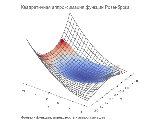
We optimize the Gauss-Newton algorithm

In Newton's method there is one drawback - the Hesse matrix. Thanks to TensorFlow, we can calculate it in one line of code. According to the wiki, Johann Karl Friedrich Gauss made the first mention of his method in 1809. Calculating the Hessian matrix for several parameters for the least squares method could then take a lot of time. Now we can assume that the Gauss-Newton algorithm uses the approximation of the Hessian matrix through the Jacobi matrix to simplify the calculations. But from the point of view of history, this is not so: Ludwig Otto Hesse (who developed the matrix named after him) was born in 1811 - 2 years after the first mention of the algorithm. And Carl Gustav Jacobi was 5 years old.

The Gauss-Newton algorithm does not work with the loss function. It works with the residual function. $r (p)$ . This function accepts a parameter vector as input. $p$ and returns the residuals vector . In our case, the vector $p$ consists of 2 components (parameters $a$ and $b$ Rosenbrock functions), and the vector of residuals from $m$ component (by the number of experiments). It turns out the vector function of the vector argument. Its derivative is:

Jacobi Matrix (vector entered - vector left)

Consider a function that accepts a vector as input and also produces a vector: $f: \ mathbb {R} ^ {N} \ rightarrow \ mathbb {R} ^ {M}$ . Derivative $f$ at the point $x$ now has size $N \ times M$ , is called the Jacobi matrix , and consists of all combinations of partial derivatives:

$\ boldsymbol {J} y_ {x} = \ begin {pmatrix} \ frac {\ partial y_ {1}} {\ partial x_ {1}} & \ cdots & \ frac {\ partial y_ {1}} {\ partial x_ {N}} \\ \ vdots & \ ddots & \ vdots \\ \ frac {\ partial y_ {M}} {\ partial x_ {1}} & \ cdots & \ frac {\ partial y_ {M}} {\ partial x_ {N}} \ end {pmatrix}$

You may notice that the rows of the Jacobi matrix are the gradients of the components $y$ . Element $(i, j)$ matrices $\ frac {\ partial y} {\ partial x}$ equals $\ frac {\ partial y_ {i}} {\ partial x_ {j}}$ and tells us how much to change $y_ {i}$ , when it changes $x_ {j}$ by a small value. As in the previous cases, you can write:

$x \ rightarrow x + \ Delta x \ Rightarrow y \ rightarrow \ approx y + \ boldsymbol {J} y_ {x} \ Delta x$

Here $\ boldsymbol {J} y_ {x}$ matrix $N \ times M$ , but $\ Delta x$ size vector $N$ so the product $\ boldsymbol {J} y_ {x} \ Delta x$ Is the product of a matrix and a vector, which results in a size vector $M$ .

In order not to be confused in the abundance of symbols, we will assume that $\ boldsymbol {J} _ {r}$ - Jacobi matrix of the function of residuals at the current point $\ boldsymbol {p}$ . Then the Gauss-Newton algorithm can be written as:

$\ boldsymbol {p} \ rightarrow \ boldsymbol {p} - [\ boldsymbol {J} _ {r} ^ \ intercal \ boldsymbol {J} _ {r}] ^ {- 1} \ boldsymbol {J} _ {r } ^ \ intercal r (\ boldsymbol {p})$

Record on the form completely coincides with the record of Newton's method. Only instead of the matrix Hesse is used $\ boldsymbol {J} _ {r} ^ \ intercal \ boldsymbol {J} _ {r}$ instead of gradient $\ boldsymbol {J} _ {r} ^ \ intercal r (\ boldsymbol {p})$ . Next, let's see why you can use such an approximation. In the meantime, let's start implementing on TensorFlow:

 #  ,  TensorFlow     , #   ,        #  .  ,   : # 1)       tf.unstack(r) # 2)      tf.gradients(r_i, p) # 3)       tf.stack #      ,     #       j = tf.stack([tf.gradients(r_i, p)[0] for r_i in tf.unstack(r)]) jT = tf.transpose(j) #     - r_col = tf.expand_dims(r, -1) #      hess_approx = tf.matmul(jT, j) grad_approx = tf.matmul(jT, r_col) # ,      dp = tf.matmul(tf.linalg.inv(hess_approx), grad_approx) #  -  - dp = tf.squeeze(dp) #  p  dp    ng = opt.apply_gradients([(dp, p)]) #   ,    40000  session.run(tf.global_variables_initializer()) train(1e-10, 40000, loss, ng, feed_dict)

 [Out]: step: 1, current loss: 3868.2291666666665 step: 2, current loss: 14.653025157673625 step: 4, current loss: 4.3918079172783016e-07 ENDED ON STEP: 4, FINAL LOSS: 3.374364957618591e-17 PARAMETERS: [2.5 2.5]

Enough 4 steps. Less than for Newton's method.

As can be seen from the code, the loss function is not used during optimization, only for the stopping and logging criteria. How does the optimization algorithm know which function to minimize? The answer is amazing: no way! Gauss-Newton minimizes only mean squared error .

We fix the mathematical part of the article

We repeated all the math we needed. Let's fix it up a bit to concentrate on programming and TensorFlow only. You may need a pencil to trace the sequence of mathematical operations.

There is a model $y = f (x, p)$ where $x$ - vector $p$ - vector of dimension parameters $n$ , but $y$ - scalar. From the experiments received $m$ points $(x_ {1}, y_ {1}), ..., (x_ {m}, y_ {m})$ ( data pairs ). The vector function of residuals depends only on the vector of parameters: $r (p) = (r_ {1} (p), ... r_ {m} (p))$ where $r_ {k} (p) = y_ {k} - \ widehat {y_ {k}} = y_ {k} - f (x_ {k}, p)$ . , $p$ , $x_{k}, y_{k}$ ? , $x_{k}, y_{k}$ , .

$p$ , ( sum of squared error — sse residual sum-of-squares — rss ) . mse sse , $m$ . . :

$loss(p) = r_{1}^2(p) + \cdots + r_{m}^2(p) = \sum_{k=1}^{m} r_{k}^2(p)$

$p$ $(p)$ .

, . — . — , $r^2$ $2r \frac{\partial r}{\partial p}$ . :

$\nabla_{p}loss = (\sum_{k=1}^{m}2r_{k}\frac{\partial r_{k}}{\partial p_{1}}, \cdots, \sum_{k=1}^{m}2r_{k}\frac{\partial r_{k}}{\partial p_{n}})$

. :

$[\boldsymbol{H}loss_{p}]_{ij} = \frac{\partial^2 loss}{\partial p_{i} \partial p_{j}} = \sum_{k=1}^{m}(2\frac{\partial r_{k}}{\partial p_{i}}\frac{\partial r_{k}}{\partial p_{j}} + 2r_{k}\frac{\partial^2 r_{k}}{\partial p_{i}\partial p_{j}})$

. , , ${(uv)}'={u}'v+u{v}'$ .
Fine! .

, , , — $2r_{k}\frac{\partial^2 r_{k}}{\partial p_{i}\partial p_{j}}$ . , , $r_{k}$ , . — . , ? -.

$\boldsymbol{J}_{r} = \begin{pmatrix} \frac{\partial r_{1}}{\partial p_{1}} & \cdots & \frac{\partial r_{1}}{\partial p_{n}}\\ \vdots & \ddots & \vdots \\ \frac{\partial r_{m}}{\partial p_{1}} & \cdots & \frac{\partial p_{m}}{\partial p_{n}} \end{pmatrix}$

, , . , :

$2\boldsymbol{J}_{r}^\intercal\boldsymbol{J}_{r} \approx \boldsymbol{H}loss_{p}$

"" . ( ). , — $2r_{k}\frac{\partial^2 r_{k}}{\partial p_{i}\partial p_{j}}$ , .
( ):

$2\boldsymbol{J}_{r}^\intercal r = \nabla_{p}loss$

, , - — , mse .

. , , . $m$ $(x_{1}, y_{1}), ..., (x_{m}, y_{m})$ , $y = rosenbrock(x, p)$ . $p$ , .

, : " . - ! ". , , , ( supervised learning ). , . : ( training set ) — ; — ( prediction model ) ; — , .

( multi-layer perceptron neural network mlp ). , , :

( starting values ) . Xavier'a, .
( overfitting ). — . , . — .
( scaling of the input ). , .

9 . 500:

 #    def get_random_rosenbrock_data_points(m): result = np.zeros((m, 3)) result[:, 0] = np.random.uniform(-2, 2, m) result[:, 1] = np.random.uniform(-2, 2, m) result[:, 2] = rosenbrock(result[:, 0], result[:, 1], 2.5, 2.5) return result m = 500 data_points = get_random_rosenbrock_data_points(m) # overfitting   ,      validation_data_points = get_random_rosenbrock_data_points(m)

500 . — ( learner ), ( outcome measurement ) ( features ) .

( network diagram ). MatLab:

( input ). $W$ ( weights ) 2x10, $b$ ( bias ) 10, ( activation ). () ( hidden layer ) 10 . , , ( output ).

, , ( $tanh$ ):

$\begin{matrix} h_{1} = tanh(xW_{1} + b_{1})\\ \widehat{y} = h_{1}W_{2} + b_{2} \end{matrix}$

$h_1 = tanh(\begin{bmatrix} x_1 & x_2 \end{bmatrix}\begin{bmatrix} w^{(1)}_{1,1} & \cdots& w^{(1)}_{1,10} \\ w^{(1)}_{2,1} &\cdots& w^{(1)}_{2,10} \end{bmatrix} + \begin{bmatrix} b^{(1)}_1 & \cdots & b^{(1)}_{10} \end{bmatrix}) \\ \widehat{y} = \begin{bmatrix}h^{(1)}_1 & \cdots & h^{(1)}_{10}\end{bmatrix} \begin{bmatrix} w^{(2)}_{1,1} \\ \vdots \\ w^{(2)}_{1,10} \\ \end{bmatrix} + b_2$

. $W_{1}$ "" $h_{1}$ , - $W_{2}$ . 41 . , .

$m \times 2$ , . - $\widehat{y}$ of $m$ :

 #     10 "" n_hidden = 10 #      Xavier'a initializer = tf.contrib.layers.xavier_initializer() #    x = tf.placeholder(tf.float64, shape=[m, 2]) y = tf.placeholder(tf.float64, shape=[m, 1]) #         W1 = tf.Variable(initializer([2, n_hidden], dtype=tf.float64)) b1 = tf.Variable(initializer([1, n_hidden], dtype=tf.float64)) #   ,  tanh   h1 = tf.nn.tanh(tf.matmul(x, W1) + b1) #        W2 = tf.Variable(initializer([n_hidden, 1], dtype=tf.float64)) b2 = tf.Variable(initializer([1], dtype=tf.float64)) #   y_hat = tf.matmul(h1, W2) + b2 #  r = y - y_hat #   mse     loss = tf.reduce_mean(tf.square(r)) #      placeholder feed_dict = {x: data_points[:,0:2], y: data_points[:,2:3]} validation_feed_dict = {x: validation_data_points[:,0:2], y: validation_data_points[:,2:3]}

Adam

Adam $rosenbrock$ . mse :

 #    adm = tf.train.AdamOptimizer(1e-2).minimize(loss) session.run(tf.global_variables_initializer()) #   ,    40000  train(1e-10, 40000, loss, adm, feed_dict) print('VALIDATION LOSS: '+str(session.run(loss, validation_feed_dict)))

 [Out]: step: 1, current loss: 671.4242576535694 [...] ENDED ON STEP: 40000, FINAL LOSS: 0.22862158574440725 VALIDATION LOSS: 0.29000289644978866

. : , , .

$rosenbrock$ 2 . :

. 9 , 500. .
. - $p$ , .

 #      y   x def jacobian(y, x): loop_vars = [ tf.constant(0, tf.int32), tf.TensorArray(tf.float64, size=m), ] #  -   #      _, jacobian = tf.while_loop( lambda i, _: i < m, #           #   (-),   x     lambda i, res: (i+1, res.write(i, tf.reshape(tf.gradients(y[i], x), (-1,)))), loop_vars) #       return jacobian.stack() #       r_flat = tf.squeeze(r) #        #       parms = [W1, b1, W2, b2] parms_sizes = [tf.size(p) for p in parms] j = tf.concat([jacobian(r_flat, p) for p in parms], 1) jT = tf.transpose(j) #           hess_approx = tf.matmul(jT, j) grad_approx = tf.matmul(jT, r)

$\boldsymbol{J}r_{p}$ . , 4 $W_1, b_1, W_2, b_2$ . 4 $\boldsymbol{J}r_{W_1}, \boldsymbol{J}r_{b_1}, \boldsymbol{J}r_{W_2}, \boldsymbol{J}r_{b_2}$ tf.concat .

. tf.while_loop , $r_i$ , , stack .

$r_i$ $W_1$ : $\begin{bmatrix} \frac{\partial r_i}{\partial w^{(1)}_{1,1}} & \cdots& \frac{\partial r_i}{\partial w^{(1)}_{1,10}} \\ \frac{\partial r_i}{\partial w^{(1)}_{2,1}} & \cdots& \frac{\partial r_i}{\partial w^{(1)}_{2,10}} \end{bmatrix}$ . tf.reshape (-1,) $\begin{bmatrix} \frac{\partial r_i}{\partial w^{(1)}_{1,1}} & \cdots& \frac{\partial r_i}{\partial w^{(1)}_{1,10}} & \frac{\partial r_i}{\partial w^{(1)}_{2,1}} & \cdots& \frac{\partial r_i}{\partial w^{(1)}_{2,10}} \end{bmatrix}$ .

. - . — TensorFlow . — - - $W_1, b_1, W_2, b_2$ . -. Levenberg-Marquardt Jupyter Notebook rosenbrock_train.py . , TensorFlow . - , ( ) , , .

-

hess_approx grad_approx -. $rosenbrock$ , . :

: $\Delta \boldsymbol{p} = \begin{bmatrix}\Delta w^{(1)}_{1,1} & \cdots & \Delta w^{(1)}_{2,10} & \Delta b^{(1)}_1 & \cdots & \Delta b^{(1)}_{10} & \Delta w^{(2)}_{1,1} & \cdots & \Delta w^{(2)}_{1,10} & \Delta b_2\end{bmatrix}$
:
$\Delta W_{1} = \begin{bmatrix}\Delta w^{(1)}_{1,1} & \cdots & \Delta w^{(1)}_{2,10} \end{bmatrix}$ , $\Delta b_{1} = \begin{bmatrix} \Delta b^{(1)}_1 & \cdots & \Delta b^{(1)}_{10} \end{bmatrix}$ , $\Delta W_{2} = \begin{bmatrix} \Delta w^{(2)}_{1,1} & \cdots & \Delta w^{(2)}_{1,10} \end{bmatrix}$ , $\Delta b_{2} = \begin{bmatrix} \Delta b_2\end{bmatrix}$ .
, :
$\Delta W_{1} = \begin{bmatrix} \Delta w^{(1)}_{1,1} & \cdots & \Delta w^{(1)}_{1,10} \\ \Delta w^{(1)}_{2,1} &\cdots & \Delta w^{(1)}_{2,10} \end{bmatrix}$ , $\Delta W_{2} = \begin{bmatrix} \Delta w^{(2)}_{1,1} \\ \vdots \\ \Delta w^{(2)}_{1,10} \\ \end{bmatrix}$
.

 # 1.     dp_flat = tf.matmul(tf.linalg.inv(hess_approx), grad_approx) # 2.     dps = tf.split(dp_flat, parms_sizes, 0) # 3.     for i in range(len(dps)): dps[i] = tf.reshape(dps[i], parms[i].shape) # 4.  :       gn = opt.apply_gradients(zip(dps, parms)) #   session.run(tf.global_variables_initializer()) train(1e-10, 100, loss, gn, feed_dict)

 [Out]: step: 1, current loss: 548.8468777701685 step: 2, current loss: 49648941.340197295 InvalidArgumentError: Input is not invertible.

Something went wrong. , . - , .

, .

-

. Matlab trainlm . . MathWorks.

- : $\boldsymbol{p} \rightarrow \boldsymbol{p}-[\boldsymbol{J}_{r}^\intercal\boldsymbol{J}_{r}]^{-1}\boldsymbol{J}_{r}^\intercal r(\boldsymbol{p})$ . - :

$\boldsymbol{p} \rightarrow \boldsymbol{p}-[\boldsymbol{J}_{r}^\intercal\boldsymbol{J}_{r}+\mu \boldsymbol{I}]^{-1}\boldsymbol{J}_{r}^\intercal r(\boldsymbol{p})$

$\ mu$ $I$ $n$ ( ). $\ mu$ , -. , . , LM -.

 mu = tf.placeholder(tf.float64, shape=[1]) n = tf.add_n(parms_sizes) I = tf.eye(n, dtype=tf.float64) # 1.     dp_flat = tf.matmul(tf.linalg.inv(hess_approx + tf.multiply(mu, I)), grad_approx) # 2.     dps = tf.split(dp_flat, parms_sizes, 0) # 3.     for i in range(len(dps)): dps[i] = tf.reshape(dps[i], parms[i].shape) # 4.  :       lm = opt.apply_gradients(zip(dps, parms))

$\ mu$ ? LM - . , . , $\ mu$ , . — , mse . , :

 #       store = [tf.Variable(tf.zeros(p.shape, dtype=tf.float64)) for p in parms] #  TensorFlow       save_parms = [tf.assign(s, p) for s, p in zip(store, parms)] restore_parms = [tf.assign(p, s) for s, p in zip(store, parms)] #   mu    3. feed_dict[mu] = np.array([3.]) step = 0 session.run(tf.global_variables_initializer()) #    mse current_loss = session.run(loss, feed_dict) #    100   while current_loss > 1e-10 and step < 100: step += 1 #  1, 2, 4...   if math.log(step, 2).is_integer(): print(f'step: {step}, mu: {feed_dict[mu][0]} current loss: {current_loss}') #    session.run(save_parms) # ,     mse while True: #    session.run(lm, feed_dict) new_loss = session.run(loss, feed_dict) if new_loss > current_loss: #  -  mu  10     feed_dict[mu] *= 10 session.run(restore_parms) else: #  -  mu  10     feed_dict[mu] /= 10 current_loss = new_loss break print(f'ENDED ON STEP: {step}, FINAL LOSS: {current_loss}') print('VALIDATION LOSS: '+str(session.run(loss, validation_feed_dict)))

 [Out]: step: 1, mu: 3.0 current loss: 692.6211687622557 [...] ENDED ON STEP: 100, FINAL LOSS: 0.012346989371823602 VALIDATION LOSS: 0.01859463694102034

100 LM mse 10 , 40 .

. , . , rosenbrock_train.py .

2D . . . , " " ( curse of dimentionality , Bellman, 1961). . .

$f(\boldsymbol{x}) = \sum_{i=1}^{N-1}\left [ 100(x_{i+1} - x_{i}^2)^2 + (1-x_{i})^2 \right ], \boldsymbol{x}=[x_1 \cdots x_{N}]\in \mathbb{R}^N$

rosenbrock_train.py get_rand_rosenbrock_points .

-

- : " ! 4 , 300! ". , ( ) -. , , . - . . : ? , . . , - :

10 000 6D .
3 12, 10, 8 (311 ).
.
3.5 .

. - 2 . LM . 20 .

rosenbrock_train.py . . , .

Conclusion

, . " ", , . , . , 273 . - , .

, :

.
( ) -:
[1] Petros Drineas, Ravi Kannan, and Michael W. Mahoney. 2006. Fast Monte Carlo Algorithms for Matrices I: Approximating Matrix Multiplication. SIAM J. Comput. 36, 1 (July 2006), 132-157. DOI= http://dx.doi.org/10.1137/S0097539704442684
[2] Adelman, M., & Silberstein, M. (2018). Faster Neural Network Training with Approximate Tensor Operations. CoRR, abs/1805.08079.

, - . , . "".

Source: https://habr.com/ru/post/428183/

All Articles