Playing Mortal Kombat with TensorFlow.js
Experimenting with improvements to the Guess.js prediction model , I began to look closely at the deep learning: recurrent neural networks (RNN), in particular, LSTM, because of their “unreasonable efficiency” in the area where Guess.js works. At the same time, I started playing with convolutional neural networks (CNN), which are also often used for time series. CNN is commonly used to classify, recognize and detect images.
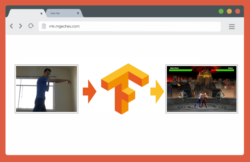
Control MK.js with TensorFlow.js
Having played with CNN, I remembered an experiment that I conducted several years ago when browser developers released the
')
The algorithm is so simple that I can explain it in a few sentences:
The video shows how the program works. GitHub source code.
Although the tiny MK clone worked successfully, the algorithm is far from perfect. Requires a frame with a background. For proper operation, the background must be the same color throughout the program. Such a restriction means that changes in light, shadows and other things will interfere and give an inaccurate result. Finally, the algorithm does not recognize actions; it classifies the new frame only as a body position from a predefined set.
Now, thanks to the progress in the web API, namely WebGL, I decided to return to this task by applying TensorFlow.js.
In this article, I will share the experience of creating a body position classification algorithm using TensorFlow.js and MobileNet. Consider the following topics:
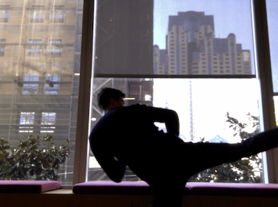
In this article, we will reduce the problem to determining the position of the body on the basis of one frame, as opposed to recognizing an action by a sequence of frames. We will develop a model of deep learning with a teacher, which, based on the image from the user's webcam, determines the movements of a person: a punch, kick or none of this.
By the end of the article we will be able to build a model for playing MK.js :

For a better understanding of the article, the reader should be familiar with the basic concepts of programming and JavaScript. A basic understanding of deep learning is also helpful, but not necessary.
The accuracy of the deep learning model largely depends on the quality of the data. We must strive to collect an extensive set of data, as in production.
Our model should be able to recognize punches and kicks. This means that we must collect images of three categories:
In this experiment, two volunteers helped me to collect photos ( @lili_vs and @gsamokovarov ). We recorded 5 QuickTime videos on my MacBook Pro, each containing 2–4 punches and 2–4 kicks.
Then we use ffmpeg to extract individual frames from videos and save them as
To run the above command, you first need to install
If we want to train a model, we must provide input data and corresponding output data, but at this stage we only have a bunch of images of three people in different poses. To structure the data, you need to classify frames in three categories: punches, kicks, and others. For each category, a separate directory is created where all relevant images are moved.
Thus, each directory should have about 200 images similar to the ones below:

Please note that there will be much more images in the Others catalog, because relatively few frames contain photos of punches and kicks, while in the remaining frames people walk, turn around or control the video. If we have too many images of one class, then we risk teaching a model biased to this particular class. In this case, when classifying an image with a blow, the neural network can still determine the class “Others”. To reduce this bias, you can remove some photos from the Others directory and train the model in an equal number of images from each category.
For convenience, we assign images in catalogs numbers from
If we train the model only on 600 photographs taken in the same environment with the same people, we will not reach a very high level of accuracy. To get the most out of our data, it’s better to generate a few extra samples using data augmentation.
Data augmentation is a technique that increases the number of data points by synthesizing new points from an existing set. Usually augmentation is used to increase the size and variety of the training set. We transfer the original images to the transformation pipeline that creates new images. You can not be too aggressive approach to transformation: from a punch should be generated only other punches.
Acceptable transformations are rotation, color inversion, blur, etc. There are excellent open source tools for augmentation of data. At the time of writing the article on JavaScript there were not too many options, so I used the library implemented in Python - imgaug . It has a set of augmenters that can be applied probabilistically.
Here is the data augmentation logic for this experiment:
This script uses the
After that, we read the image from the disk and apply a number of transformations to it. I have documented most of the transformations in the above code snippet, so we will not repeat.
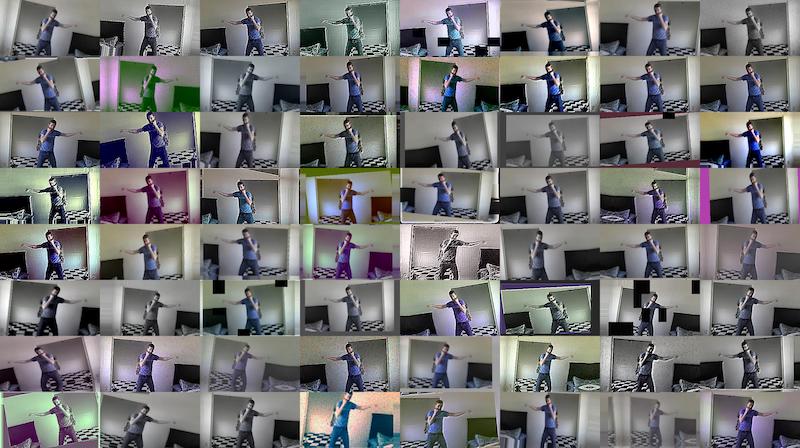
For each image creates 16 other images. Here is an example of what they look like:
Please note that in the above script, we scale images up to
Now we will build a model for classification!
Since we are dealing with images, we use the convolutional neural network (CNN). This network architecture is known to be suitable for image recognition, object detection and classification.
The image below shows the popular CNN VGG-16 used to classify images.
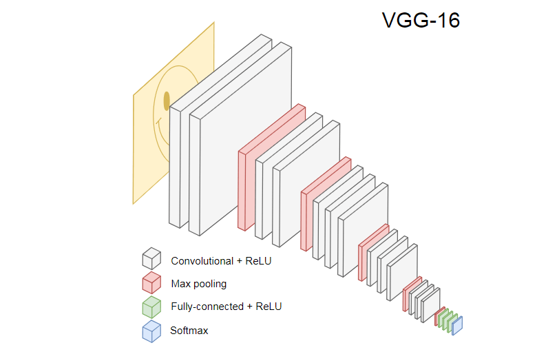
The neural VGG-16 recognizes 1000 image classes. It has 16 layers (not counting the pooling layers and the output). This multi-layer network is difficult to train in practice. This will require a large data set and many hours of training.
The hidden layers of the trained CNN recognize the various elements of the images from the training set, starting at the edges, moving on to more complex elements, such as figures, individual objects, and so on. A trained CNN-style VGG-16 for recognizing a large set of images should have hidden layers that have learned many features from the training set. Such signs will be common to most images and, accordingly, be reused for different tasks.
Transfer learning allows you to reuse an existing and trained network. We can take the output from any of the layers of the existing network and transmit it as input to the new neural network. Thus, by teaching the newly created neural network, over time it can be taught to recognize new features of a higher level and correctly classify images from classes that the original model has never seen before.
For our purposes, let's take the MobileNet neural network from the @ tensorflow-models / mobilenet package . MobileNet is just as powerful as VGG-16, but it is much smaller, which speeds up forward propagation, that is, network activation (forward propagation), and reduces download time in the browser. MobileNet trained on a data set for image classification ILSVRC-2012-CLS .
When developing a model with a transfer of training, we have choices for two points:
The first moment is very significant. Depending on the selected layer, we will get the signs at a lower or higher level of abstraction as input for our neural network.
We are not going to train any layers of MobileNet. Select the output from
The initial task was to classify the image into three classes: hand, foot and other movements. Let's first solve the problem of a smaller one: determine whether there is a punch in the frame or not. This is a typical binary classification task. For this purpose, we can define the following model:
This code defines a simple model, a layer with
Why did I choose
The
If you transfer training from the original MobileNet model, you first need to download it. Since it is impractical to train our model on more than 3000 images in the browser, we will apply Node.js and load the neural network from the file.
Download MobileNet here . The catalog contains the
Note that in the
Now you need to create a data set for learning the model. To do this, we have to skip all the images through the
In the code above, we first read the files in the directories with and without hitting. Then we determine the one-dimensional tensor containing the output labels. If we have
In
As a result, for each
Now the model is ready to learn! Call the
The above code calls
The size of the package determines the
After running the training script, you will see a result similar to the one below:
Notice how accuracy increases over time, and loss decreases.
On my data set, the model after training showed an accuracy of 92%. Keep in mind that accuracy may not be very high due to the small set of training data.
In the previous section, we trained the binary classification model. Now run it in the browser and connect it to the game MK.js !
In the given code there are several declarations:
After that we get the video stream from the user's camera and set it as the source for the item
The next step is to implement a grayscale filter that accepts
As a next step, let's link the model with MK.js:
In the code above, we first load the model that was trained above, and then load MobileNet. Pass MobileNet to the method
The most interesting begins in the method
The next step is to transfer the frame to MobileNet, get the output from the desired hidden layer and transfer it as input to the method of
Finally, we check: if the probability of a hand strike exceeds
Done! Here is the result!

In the next section, we will make a smarter model: a neural network that recognizes punches, kicks, and other images. This time we start with the preparation of the training set:
As before, we first read the catalogs with the images of punches by hand, foot and other images. After that, unlike last time, we form the expected result in the form of a two-dimensional tensor, but not a one-dimensional one. If we have n pictures with a punch, m pictures with a kick and k other images, then in the tensor there
A vector of
After that we form the input tensor
There will have to update the definition of the model:
The only two differences from the previous model are:
There are three units in the output layer, because we have three different categories of images:
Activation is triggered on these three units
After learning the model over the
The next step is to launch the model in the browser! Since the logic is very similar to running the model for binary classification, take a look at the last step, where an action is chosen based on the model output:
First we call MobileNet with a reduced frame in shades of gray, then we transfer the result of our trained model. The model returns a one-dimensional tensor, which we convert to
If the probability of the third result exceeds
In general, that's all! The result is shown below:

If you collect a large and diverse set of data about people who hit with arms and legs, then you can build a model that works perfectly on individual frames. But is that enough? What if we want to go even further and distinguish two different types of kicks: with a turn and from the back (back kick).
As can be seen on the frames below, at a certain point in time from a certain angle, both hits look the same:

But if you look at the execution, the movements are completely different:
How can you teach the neural network to analyze the sequence of frames, and not just one frame?
For this purpose, we can explore another class of neural networks, called recurrent neural networks (RNN). For example, RNN is great for working with time series:
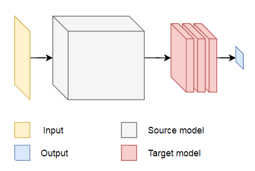
Implementing such a model is beyond the scope of this article, but let's look at an example of architecture in order to get an idea of how all this will work together.
The diagram below shows the recognition model of actions:
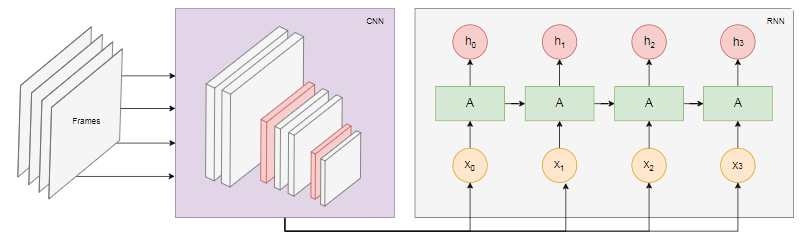
Take the last
In this article, we developed an image classification model. For this purpose, we collected a data set: extracted video frames and manually divided them into three categories. Then augmented the data by adding images using imgaug .
After that, we explained what training transfer is and used the trained MobileNet model from the @ tensorflow-models / mobilenet package for our own purposes . We loaded MobileNet from a file in the Node.js process and trained an extra dense layer where data was fed from the hidden MobileNet layer. After training, we have reached an accuracy of more than 90%!
To use this model in the browser, we downloaded it together with MobileNet and ran a frame categorization from the user's webcam every 100 ms. We connected the model with the game.MK.js and used the output of the model to control one of the characters.
Finally, we looked at how to improve the model by combining it with a recurrent neural network to recognize actions.
I hope you enjoyed this tiny project as much as I did!
Control MK.js with TensorFlow.js
The source code for this article and MK.js are on my GitHub . I have not laid out the training data set, but you can build your own and train the model as described below!
Having played with CNN, I remembered an experiment that I conducted several years ago when browser developers released the
getUserMedia API. In it, the user's camera served as a controller for playing a small JavaScript-clone of Mortal Kombat 3. You can find that game in the GitHub repository . As part of the experiment, I implemented a basic positioning algorithm, which classifies an image into the following classes:')
- Blow left or right hand
- Kick left or right foot
- Steps left and right
- Squat
- None of the above
The algorithm is so simple that I can explain it in a few sentences:
The algorithm photographs the background. As soon as the user appears in the frame, the algorithm calculates the difference between the background and the current frame with the user. So he determines the position of the user's figure. The next step is to display the user's body in white on black. After that, vertical and horizontal histograms are constructed, summarizing the values for each pixel. Based on this calculation, the algorithm determines the current body position.
The video shows how the program works. GitHub source code.
Although the tiny MK clone worked successfully, the algorithm is far from perfect. Requires a frame with a background. For proper operation, the background must be the same color throughout the program. Such a restriction means that changes in light, shadows and other things will interfere and give an inaccurate result. Finally, the algorithm does not recognize actions; it classifies the new frame only as a body position from a predefined set.
Now, thanks to the progress in the web API, namely WebGL, I decided to return to this task by applying TensorFlow.js.
Introduction
In this article, I will share the experience of creating a body position classification algorithm using TensorFlow.js and MobileNet. Consider the following topics:
- Collection of training data for image classification
- Data augmentation with imgaug
- Transfer training with MobileNet
- Binary classification and N-tric classification
- Learning the model for classifying images TensorFlow.js in Node.js and using it in a browser
- A few words about the classification of actions with LSTM
In this article, we will reduce the problem to determining the position of the body on the basis of one frame, as opposed to recognizing an action by a sequence of frames. We will develop a model of deep learning with a teacher, which, based on the image from the user's webcam, determines the movements of a person: a punch, kick or none of this.
By the end of the article we will be able to build a model for playing MK.js :
For a better understanding of the article, the reader should be familiar with the basic concepts of programming and JavaScript. A basic understanding of deep learning is also helpful, but not necessary.
Data collection
The accuracy of the deep learning model largely depends on the quality of the data. We must strive to collect an extensive set of data, as in production.
Our model should be able to recognize punches and kicks. This means that we must collect images of three categories:
- Hand punches
- Foot kicks
- Other
In this experiment, two volunteers helped me to collect photos ( @lili_vs and @gsamokovarov ). We recorded 5 QuickTime videos on my MacBook Pro, each containing 2–4 punches and 2–4 kicks.
Then we use ffmpeg to extract individual frames from videos and save them as
jpg images:ffmpeg -i video.mov $filename%03d.jpgTo run the above command, you first need to install
ffmpeg on your computer.If we want to train a model, we must provide input data and corresponding output data, but at this stage we only have a bunch of images of three people in different poses. To structure the data, you need to classify frames in three categories: punches, kicks, and others. For each category, a separate directory is created where all relevant images are moved.
Thus, each directory should have about 200 images similar to the ones below:
Please note that there will be much more images in the Others catalog, because relatively few frames contain photos of punches and kicks, while in the remaining frames people walk, turn around or control the video. If we have too many images of one class, then we risk teaching a model biased to this particular class. In this case, when classifying an image with a blow, the neural network can still determine the class “Others”. To reduce this bias, you can remove some photos from the Others directory and train the model in an equal number of images from each category.
For convenience, we assign images in catalogs numbers from
1 to 190 , so the first image will be 1.jpg , the second 2.jpg , etc.If we train the model only on 600 photographs taken in the same environment with the same people, we will not reach a very high level of accuracy. To get the most out of our data, it’s better to generate a few extra samples using data augmentation.
Data augmentation
Data augmentation is a technique that increases the number of data points by synthesizing new points from an existing set. Usually augmentation is used to increase the size and variety of the training set. We transfer the original images to the transformation pipeline that creates new images. You can not be too aggressive approach to transformation: from a punch should be generated only other punches.
Acceptable transformations are rotation, color inversion, blur, etc. There are excellent open source tools for augmentation of data. At the time of writing the article on JavaScript there were not too many options, so I used the library implemented in Python - imgaug . It has a set of augmenters that can be applied probabilistically.
Here is the data augmentation logic for this experiment:
np.random.seed(44) ia.seed(44) def main(): for i in range(1, 191): draw_single_sequential_images(str(i), "others", "others-aug") for i in range(1, 191): draw_single_sequential_images(str(i), "hits", "hits-aug") for i in range(1, 191): draw_single_sequential_images(str(i), "kicks", "kicks-aug") def draw_single_sequential_images(filename, path, aug_path): image = misc.imresize(ndimage.imread(path + "/" + filename + ".jpg"), (56, 100)) sometimes = lambda aug: iaa.Sometimes(0.5, aug) seq = iaa.Sequential( [ iaa.Fliplr(0.5), # horizontally flip 50% of all images # crop images by -5% to 10% of their height/width sometimes(iaa.CropAndPad( percent=(-0.05, 0.1), pad_mode=ia.ALL, pad_cval=(0, 255) )), sometimes(iaa.Affine( scale={"x": (0.8, 1.2), "y": (0.8, 1.2)}, # scale images to 80-120% of their size, individually per axis translate_percent={"x": (-0.1, 0.1), "y": (-0.1, 0.1)}, # translate by -10 to +10 percent (per axis) rotate=(-5, 5), shear=(-5, 5), # shear by -5 to +5 degrees order=[0, 1], # use nearest neighbour or bilinear interpolation (fast) cval=(0, 255), # if mode is constant, use a cval between 0 and 255 mode=ia.ALL # use any of scikit-image's warping modes (see 2nd image from the top for examples) )), iaa.Grayscale(alpha=(0.0, 1.0)), iaa.Invert(0.05, per_channel=False), # invert color channels # execute 0 to 5 of the following (less important) augmenters per image # don't execute all of them, as that would often be way too strong iaa.SomeOf((0, 5), [ iaa.OneOf([ iaa.GaussianBlur((0, 2.0)), # blur images with a sigma between 0 and 2.0 iaa.AverageBlur(k=(2, 5)), # blur image using local means with kernel sizes between 2 and 5 iaa.MedianBlur(k=(3, 5)), # blur image using local medians with kernel sizes between 3 and 5 ]), iaa.Sharpen(alpha=(0, 1.0), lightness=(0.75, 1.5)), # sharpen images iaa.Emboss(alpha=(0, 1.0), strength=(0, 2.0)), # emboss images iaa.AdditiveGaussianNoise(loc=0, scale=(0.0, 0.01*255), per_channel=0.5), # add gaussian noise to images iaa.Add((-10, 10), per_channel=0.5), # change brightness of images (by -10 to 10 of original value) iaa.AddToHueAndSaturation((-20, 20)), # change hue and saturation # either change the brightness of the whole image (sometimes # per channel) or change the brightness of subareas iaa.OneOf([ iaa.Multiply((0.9, 1.1), per_channel=0.5), iaa.FrequencyNoiseAlpha( exponent=(-2, 0), first=iaa.Multiply((0.9, 1.1), per_channel=True), second=iaa.ContrastNormalization((0.9, 1.1)) ) ]), iaa.ContrastNormalization((0.5, 2.0), per_channel=0.5), # improve or worsen the contrast ], random_order=True ) ], random_order=True ) im = np.zeros((16, 56, 100, 3), dtype=np.uint8) for c in range(0, 16): im[c] = image for im in range(len(grid)): misc.imsave(aug_path + "/" + filename + "_" + str(im) + ".jpg", grid[im]) This script uses the
main method with three for loops — one for each category of images. In each iteration, in each of the cycles, we call the draw_single_sequential_images method: the first argument is the file name, the second is the path, and the third is the directory where to save the result.After that, we read the image from the disk and apply a number of transformations to it. I have documented most of the transformations in the above code snippet, so we will not repeat.
For each image creates 16 other images. Here is an example of what they look like:
Please note that in the above script, we scale images up to
100x56 pixels. We do this to reduce the amount of data and, accordingly, the number of calculations that our model performs during training and evaluation.Model building
Now we will build a model for classification!
Since we are dealing with images, we use the convolutional neural network (CNN). This network architecture is known to be suitable for image recognition, object detection and classification.
Transfer training
The image below shows the popular CNN VGG-16 used to classify images.
The neural VGG-16 recognizes 1000 image classes. It has 16 layers (not counting the pooling layers and the output). This multi-layer network is difficult to train in practice. This will require a large data set and many hours of training.
The hidden layers of the trained CNN recognize the various elements of the images from the training set, starting at the edges, moving on to more complex elements, such as figures, individual objects, and so on. A trained CNN-style VGG-16 for recognizing a large set of images should have hidden layers that have learned many features from the training set. Such signs will be common to most images and, accordingly, be reused for different tasks.
Transfer learning allows you to reuse an existing and trained network. We can take the output from any of the layers of the existing network and transmit it as input to the new neural network. Thus, by teaching the newly created neural network, over time it can be taught to recognize new features of a higher level and correctly classify images from classes that the original model has never seen before.
For our purposes, let's take the MobileNet neural network from the @ tensorflow-models / mobilenet package . MobileNet is just as powerful as VGG-16, but it is much smaller, which speeds up forward propagation, that is, network activation (forward propagation), and reduces download time in the browser. MobileNet trained on a data set for image classification ILSVRC-2012-CLS .
When developing a model with a transfer of training, we have choices for two points:
- The output from which layer of the source model to use as input for the target model.
- How many layers of the target model are we going to train, if any.
The first moment is very significant. Depending on the selected layer, we will get the signs at a lower or higher level of abstraction as input for our neural network.
We are not going to train any layers of MobileNet. Select the output from
global_average_pooling2d_1 and pass it as input to our tiny model. Why did I choose this particular layer? Empirically. I did some tests and this layer works quite well.Model definition
The initial task was to classify the image into three classes: hand, foot and other movements. Let's first solve the problem of a smaller one: determine whether there is a punch in the frame or not. This is a typical binary classification task. For this purpose, we can define the following model:
import * as tf from '@tensorflow/tfjs'; const model = tf.sequential(); model.add(tf.layers.inputLayer({ inputShape: [1024] })); model.add(tf.layers.dense({ units: 1024, activation: 'relu' })); model.add(tf.layers.dense({ units: 1, activation: 'sigmoid' })); model.compile({ optimizer: tf.train.adam(1e-6), loss: tf.losses.sigmoidCrossEntropy, metrics: ['accuracy'] }); This code defines a simple model, a layer with
1024 units and ReLU activation, as well as one output unit that passes through the sigmoid activation sigmoid . The latter gives a number from 0 to 1 , depending on the probability of the presence of a hand strike in a given frame.Why did I choose
1024 units for the second level and learning speed 1e-6 ? Well, I tried several different options and saw that such parameters work best. The “spear method” does not seem to be the best approach, but to a large extent this is exactly how setting up hyper parameters in deep learning - based on our understanding of the model, we use intuition to update orthogonal parameters and empirically check how the model works.The
compile method compiles the layers together, preparing a model for learning and evaluation. Here we announce that we want to use the adam optimization algorithm. We also declare that we will calculate the loss (loss) from the cross entropy, and indicate that we want to evaluate the accuracy of the model. Then TensorFlow.js calculates the accuracy by the formula:Accuracy = (True Positives + True Negatives) / (Positives + Negatives)If you transfer training from the original MobileNet model, you first need to download it. Since it is impractical to train our model on more than 3000 images in the browser, we will apply Node.js and load the neural network from the file.
Download MobileNet here . The catalog contains the
model.json file, which contains the model architecture - layers, activations, etc. The remaining files contain the parameters of the model. You can load a model from a file using this code: export const loadModel = async () => { const mn = new mobilenet.MobileNet(1, 1); mn.path = `file://PATH/TO/model.json`; await mn.load(); return (input): tf.Tensor1D => mn.infer(input, 'global_average_pooling2d_1') .reshape([1024]); }; Note that in the
loadModel method loadModel we return a function that takes a one-dimensional tensor as input and returns mn.infer(input, Layer) . The infer method takes a tensor and a layer as arguments. The layer determines which hidden layer we want to get the output from. If you open model.json and global_average_pooling2d_1 , you will find this name in one of the layers.Now you need to create a data set for learning the model. To do this, we have to skip all the images through the
infer method in MobileNet and assign them tags: 1 for images with strokes and 0 for images without impact: const punches = require('fs') .readdirSync(Punches) .filter(f => f.endsWith('.jpg')) .map(f => `${Punches}/${f}`); const others = require('fs') .readdirSync(Others) .filter(f => f.endsWith('.jpg')) .map(f => `${Others}/${f}`); const ys = tf.tensor1d( new Array(punches.length).fill(1) .concat(new Array(others.length).fill(0))); const xs: tf.Tensor2D = tf.stack( punches .map((path: string) => mobileNet(readInput(path))) .concat(others.map((path: string) => mobileNet(readInput(path)))) ) as tf.Tensor2D; In the code above, we first read the files in the directories with and without hitting. Then we determine the one-dimensional tensor containing the output labels. If we have
n images with hits and m other images, the tensor will have n elements with a value of 1 and m elements with a value of 0.In
xs we add the results of calling the infer method for individual images. Notice that for each image we call the readInput method. Here is its implementation: export const readInput = img => imageToInput(readImage(img), TotalChannels); const readImage = path => jpeg.decode(fs.readFileSync(path), true); const imageToInput = image => { const values = serializeImage(image); return tf.tensor3d(values, [image.height, image.width, 3], 'int32'); }; const serializeImage = image => { const totalPixels = image.width * image.height; const result = new Int32Array(totalPixels * 3); for (let i = 0; i < totalPixels; i++) { result[i * 3 + 0] = image.data[i * 4 + 0]; result[i * 3 + 1] = image.data[i * 4 + 1]; result[i * 3 + 2] = image.data[i * 4 + 2]; } return result; }; readInput first calls the readImage function, and then delegates its imageToInput call. The readImage function reads the image from the disk and then decodes the jpg from the buffer using the jpeg-js package. In imageToInput we transform the image into a three-dimensional tensor.As a result, for each
i from 0 to TotalImages , ys[i] should be equal to 1 if xs[i] corresponds to the image with a stroke, and 0 otherwise.Model training
Now the model is ready to learn! Call the
fit method: await model.fit(xs, ys, { epochs: Epochs, batchSize: parseInt(((punches.length + others.length) * BatchSize).toFixed(0)), callbacks: { onBatchEnd: async (_, logs) => { console.log('Cost: %s, accuracy: %s', logs.loss.toFixed(5), logs.acc.toFixed(5)); await tf.nextFrame(); } } }); The above code calls
fit with three arguments: xs , ys and a configuration object. In the configuration object, we set how many epochs the model will study, the packet size, and the callback that TensorFlow.js will generate after processing each packet.The size of the package determines the
xs and ys for training the model for the same epoch. For each epoch, TensorFlow.js will select a subset of xs and the corresponding elements from ys , perform a direct distribution, obtain the output of the layer with sigmoid activation, and then, based on the loss, perform optimization using the adam algorithm.After running the training script, you will see a result similar to the one below:
  Cost: 0.84212, accuracy: 1.00000
 eta = 0.3> ---------- acc = 1.00 loss = 0.84 Cost: 0.79740, accuracy: 1.00000
 eta = 0.2 => --------- acc = 1.00 loss = 0.80 Cost: 0.81533, accuracy: 1.00000
 eta = 0.2 ==> -------- acc = 1.00 loss = 0.82 Cost: 0.64303, accuracy: 0.50000
 eta = 0.2 ===> ------- acc = 0.50 loss = 0.64 Cost: 0.51377, accuracy: 0.00000
 eta = 0.2 ====> ------ acc = 0.00 loss = 0.51 Cost: 0.46473, accuracy: 0.50000
 eta = 0.1 =====> ----- acc = 0.50 loss = 0.46 Cost: 0.50872, accuracy: 0.00000
 eta = 0.1 ======> ---- acc = 0.00 loss = 0.51 Cost: 0.62556, accuracy: 1.00000
 eta = 0.1 =======> --- acc = 1.00 loss = 0.63 Cost: 0.65133, accuracy: 0.50000
 eta = 0.1 ========> - acc = 0.50 loss = 0.65 Cost: 0.63824, accuracy: 0.50000
 eta = 0.0 ==========>
 293ms 14675us / step - acc = 0.60 loss = 0.65
 Epoch 3/50
 Cost: 0.44661, accuracy: 1.00000
 eta = 0.3> ---------- acc = 1.00 loss = 0.45 Cost: 0.78060, accuracy: 1.00000
 eta = 0.3 => --------- acc = 1.00 loss = 0.78 Cost: 0.79208, accuracy: 1.00000
 eta = 0.3 ==> -------- acc = 1.00 loss = 0.79 Cost: 0.49072, accuracy: 0.50000
 eta = 0.2 ===> ------- acc = 0.50 loss = 0.49 Cost: 0.62232, accuracy: 1.00000
 eta = 0.2 ====> ------ acc = 1.00 loss = 0.62 Cost: 0.82899, accuracy: 1.00000
 eta = 0.2 =====> ----- acc = 1.00 loss = 0.83 Cost: 0.67629, accuracy: 0.50000
 eta = 0.1 ======> ---- acc = 0.50 loss = 0.68 Cost: 0.62621, accuracy: 0.50000
 eta = 0.1 =======> --- acc = 0.50 loss = 0.63 Cost: 0.46077, accuracy: 1.00000
 eta = 0.1 ========> - acc = 1.00 loss = 0.46 Cost: 0.62076, accuracy: 1.00000
 eta = 0.0 ==========>
 304ms 15221us / step - acc = 0.85 loss = 0.63
Notice how accuracy increases over time, and loss decreases.
On my data set, the model after training showed an accuracy of 92%. Keep in mind that accuracy may not be very high due to the small set of training data.
Running the model in a browser
In the previous section, we trained the binary classification model. Now run it in the browser and connect it to the game MK.js !
const video = document.getElementById('cam'); const Layer = 'global_average_pooling2d_1'; const mobilenetInfer = m => (p): tf.Tensor<tf.Rank> => m.infer(p, Layer); const canvas = document.getElementById('canvas'); const scale = document.getElementById('crop'); const ImageSize = { Width: 100, Height: 56 }; navigator.mediaDevices .getUserMedia({ video: true, audio: false }) .then(stream => { video.srcObject = stream; }); In the given code there are several declarations:
videocontains a link to theHTML5 videoelement on the page.Layercontains the name of the layer from MobileNet, from which we want to get the output data and transfer them as input data for our modelmobilenetInfer- A function that accepts a MobileNet instance and returns another function. The return function takes the input data and returns the corresponding output from the specified MobileNet layer.canvaspoints to the elementHTML5 canvaswe will use to extract frames from the videoscale- another onecanvasthat is used to scale individual frames
After that we get the video stream from the user's camera and set it as the source for the item
video.The next step is to implement a grayscale filter that accepts
canvasand converts its contents: const grayscale = (canvas: HTMLCanvasElement) => { const imageData = canvas.getContext('2d').getImageData(0, 0, canvas.width, canvas.height); const data = imageData.data; for (let i = 0; i < data.length; i += 4) { const avg = (data[i] + data[i + 1] + data[i + 2]) / 3; data[i] = avg; data[i + 1] = avg; data[i + 2] = avg; } canvas.getContext('2d').putImageData(imageData, 0, 0); }; As a next step, let's link the model with MK.js:
let mobilenet: (p: any) => tf.Tensor<tf.Rank>; tf.loadModel('http://localhost:5000/model.json').then(model => { mobileNet .load() .then((mn: any) => mobilenet = mobilenetInfer(mn)) .then(startInterval(mobilenet, model)); }); In the code above, we first load the model that was trained above, and then load MobileNet. Pass MobileNet to the method
mobilenetInferto get the path to calculate the output from the hidden network layer. After that we call the method startIntervalwith two networks as arguments. const startInterval = (mobilenet, model) => () => { setInterval(() => { canvas.getContext('2d').drawImage(video, 0, 0); grayscale(scale .getContext('2d') .drawImage( canvas, 0, 0, canvas.width, canvas.width / (ImageSize.Width / ImageSize.Height), 0, 0, ImageSize.Width, ImageSize.Height )); const [punching] = Array.from(( model.predict(mobilenet(tf.fromPixels(scale))) as tf.Tensor1D) .dataSync() as Float32Array); const detect = (window as any).Detect; if (punching >= 0.4) detect && detect.onPunch(); }, 100); }; The most interesting begins in the method
startInterval! First, we start the interval, where every 100mscall an anonymous function. It first canvasrenders the video with the current frame. Then we reduce the frame size before 100x56and apply a gray scale filter to it.The next step is to transfer the frame to MobileNet, get the output from the desired hidden layer and transfer it as input to the method of
predictour model. That returns a tensor with one element. With the help dataSyncwe get the value from the tensor and assign it to a constant punching.Finally, we check: if the probability of a hand strike exceeds
0.4, then we call the onPunchglobal object method Detect. MK.js provides a global object with three methods:onKick, onPunchand onStandthat we can use to control one of the characters.Done! Here is the result!
Recognition of kicking and kicking with N-striking classification
In the next section, we will make a smarter model: a neural network that recognizes punches, kicks, and other images. This time we start with the preparation of the training set:
const punches = require('fs') .readdirSync(Punches) .filter(f => f.endsWith('.jpg')) .map(f => `${Punches}/${f}`); const kicks = require('fs') .readdirSync(Kicks) .filter(f => f.endsWith('.jpg')) .map(f => `${Kicks}/${f}`); const others = require('fs') .readdirSync(Others) .filter(f => f.endsWith('.jpg')) .map(f => `${Others}/${f}`); const ys = tf.tensor2d( new Array(punches.length) .fill([1, 0, 0]) .concat(new Array(kicks.length).fill([0, 1, 0])) .concat(new Array(others.length).fill([0, 0, 1])), [punches.length + kicks.length + others.length, 3] ); const xs: tf.Tensor2D = tf.stack( punches .map((path: string) => mobileNet(readInput(path))) .concat(kicks.map((path: string) => mobileNet(readInput(path)))) .concat(others.map((path: string) => mobileNet(readInput(path)))) ) as tf.Tensor2D; As before, we first read the catalogs with the images of punches by hand, foot and other images. After that, unlike last time, we form the expected result in the form of a two-dimensional tensor, but not a one-dimensional one. If we have n pictures with a punch, m pictures with a kick and k other images, then in the tensor there
yswill be nelements with a value [1, 0, 0], melements with a value, [0, 1, 0]and kelements with a value [0, 0, 1].A vector of
nelements, in which there are n - 1elements with a value 0and one element with a value 1, we call a unitary vector (one-hot vector).After that we form the input tensor
xsby folding the output of each image from MobileNet.There will have to update the definition of the model:
const model = tf.sequential(); model.add(tf.layers.inputLayer({ inputShape: [1024] })); model.add(tf.layers.dense({ units: 1024, activation: 'relu' })); model.add(tf.layers.dense({ units: 3, activation: 'softmax' })); await model.compile({ optimizer: tf.train.adam(1e-6), loss: tf.losses.sigmoidCrossEntropy, metrics: ['accuracy'] }); The only two differences from the previous model are:
- The number of units in the output layer
- Activations in the output layer
There are three units in the output layer, because we have three different categories of images:
- Punch
- Kick
- Other
Activation is triggered on these three units
softmax, which converts their parameters to a three-value tensor. Why three units for the output layer? Each of the three values for three classes can be represented by two bits: 00, 01, 10. The sum of the values of the tensor created softmaxis 1, that is, we will never get 00, so we cannot classify the images of one of the classes.After learning the model over the
500ages, I achieved an accuracy of about 92%! This is not bad, but do not forget that the training was conducted on a small set of data.The next step is to launch the model in the browser! Since the logic is very similar to running the model for binary classification, take a look at the last step, where an action is chosen based on the model output:
const [punch, kick, nothing] = Array.from((model.predict( mobilenet(tf.fromPixels(scaled)) ) as tf.Tensor1D).dataSync() as Float32Array); const detect = (window as any).Detect; if (nothing >= 0.4) return; if (kick > punch && kick >= 0.35) { detect.onKick(); return; } if (punch > kick && punch >= 0.35) detect.onPunch(); First we call MobileNet with a reduced frame in shades of gray, then we transfer the result of our trained model. The model returns a one-dimensional tensor, which we convert to
Float32Arrays dataSync. In the next step, we use Array.fromto cast a typed array to a JavaScript array. Then we extract the probabilities that there is a punch, a kick or nothing on the frame.If the probability of the third result exceeds
0.4, return. Otherwise, if the probability of a kick is higher 0.32, send a kick command to MK.js. If the probability of hitting with your hand is higher 0.32and higher than the probability of hitting with your foot, then send the action of hitting with your hand.In general, that's all! The result is shown below:
Action recognition
If you collect a large and diverse set of data about people who hit with arms and legs, then you can build a model that works perfectly on individual frames. But is that enough? What if we want to go even further and distinguish two different types of kicks: with a turn and from the back (back kick).
As can be seen on the frames below, at a certain point in time from a certain angle, both hits look the same:
But if you look at the execution, the movements are completely different:
How can you teach the neural network to analyze the sequence of frames, and not just one frame?
For this purpose, we can explore another class of neural networks, called recurrent neural networks (RNN). For example, RNN is great for working with time series:
- Natural language processing (NLP), where each word depends on the preceding and following
- Predict the next page based on your browsing history
- Recognizing actions in a sequence of frames
Implementing such a model is beyond the scope of this article, but let's look at an example of architecture in order to get an idea of how all this will work together.
Might RNN
The diagram below shows the recognition model of actions:
Take the last
nframes from the video and transfer them to CNN. The CNN output for each frame is passed as input to the RNN. The recurrent neural network will determine the dependencies between the individual frames and recognize which action they correspond to.Conclusion
In this article, we developed an image classification model. For this purpose, we collected a data set: extracted video frames and manually divided them into three categories. Then augmented the data by adding images using imgaug .
After that, we explained what training transfer is and used the trained MobileNet model from the @ tensorflow-models / mobilenet package for our own purposes . We loaded MobileNet from a file in the Node.js process and trained an extra dense layer where data was fed from the hidden MobileNet layer. After training, we have reached an accuracy of more than 90%!
To use this model in the browser, we downloaded it together with MobileNet and ran a frame categorization from the user's webcam every 100 ms. We connected the model with the game.MK.js and used the output of the model to control one of the characters.
Finally, we looked at how to improve the model by combining it with a recurrent neural network to recognize actions.
I hope you enjoyed this tiny project as much as I did!
Source: https://habr.com/ru/post/428019/
All Articles