If you don't know what color temperature is, start from here .

While working on the Color Temperature tool for PhotoDemon , I spent the whole evening trying to determine a simple and clear algorithm for the conversion between temperature values ​​(in Kelvin) and RGB. I thought that such an algorithm would be easy to find, because many photo editors have tools for correcting color temperature, and in every modern camera, including smartphones, there is an adjustment of white balance based on lighting conditions.


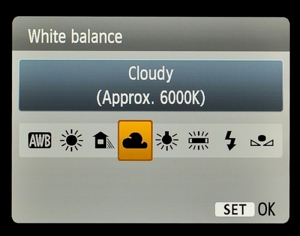
An example of a camera screen with white balance setting. A source
')
It turned out to find a reliable formula for converting temperature to RGB is almost impossible. Of course, there are some algorithms, but most of them work by converting temperature into the XYZ color space, to which you can then add an RGB conversion. Such algorithms seem to be based on the Robertson method, one implementation of which is here and the other here .

Unfortunately, this approach does not provide a purely mathematical formula - it is just an interpolation on the conversion table. This may be reasonable in certain circumstances, but when you consider the additional XYZ → RGB conversion, it turns out too slow to simply adjust the color temperature in real time.

So I wrote my own algorithm, and it works damn well. Here is how I did it.

Warnings regarding this algorithm

Warning 1 : my algorithm provides a high-quality approximation, but it is not accurate enough for serious scientific use. It is intended primarily for manipulating photographs — so do not try to use it for astronomy or medicine.

Warning 2 : Because of its relative simplicity, this algorithm is fast enough to work in real time on images of reasonable size (I tested it on 12-megapixel images), but to achieve the best results, you should apply the mathematical optimizations specific to your programming language. I show an algorithm without mathematical optimizations, so as not to complicate it.

Warning 3 : The algorithm is intended only for use in the range from 1000 K to 40000 K, which is a good range for photography. (In fact, it is much more than may be required in most situations). Although it works for temperatures outside this range, but the quality will decrease.

Special thanks to Mitchell Charity

First, I have to pay a big debt and thank Mitchell Charity for the source data that he used to create these algorithms: the raw black body file . Charity provides two data sets, and my algorithm uses the CIE 1964 10-degree color matching function . A discussion of the 2-degree function of CIE 1931 with Judd Vos corrections versus a 10-degree set is beyond the scope of this article, but if you're interested, you can start a comprehensive analysis from this page .

Algorithm: an example of issuing

Here is the output of the algorithm in the range from 1000 K to 40000 K:


The output of my algorithm is from 1000 K to 40000 K. The white dot is at 6500−6600 K, which is ideal for processing photos on a modern LCD monitor

Here is a more detailed snapshot of the algorithm in the interesting range for photography from 1500 K to 15000 K:


The same algorithm, but from 1500 K to 15000 K

As you can see, banding is minimal, which is a great improvement over the aforementioned correspondence tables. The algorithm also does a great job of preserving the light yellow tint near the white point, which is important for simulating daylight in post-processing of photos.

How I came to this algorithm

The first step to deriving a reliable formula was to plot the original black body values ​​from Charity . You can download the entire spreadsheet in the LibreOffice / OpenOffice .ods format (430 KB) .

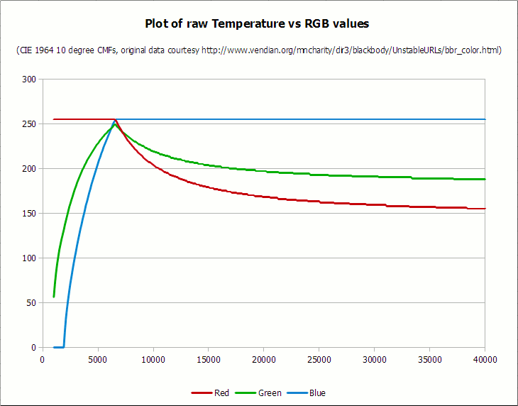
Here are the data after plotting:


Data of original temperature (K) in RGB (sRGB), graph LibreOffice Calc. Again, the conversion is based on the 10-degree CMF function of the CIE 1964. The white dot, as required, is between 6,500 K and 6,600 K (the peak is on the left side of the graph). A source

It is easy to notice that there are several sections that simplify our algorithm. In particular:

• Red values ​​below 6600 K are always 255
• Blue values ​​below 2000 K are always 0
• Blue values ​​above 6500 K are always 255

It is also important to note that in order to fit the curve to the given green color, it is best viewed as two separate curves - one for temperatures below 6600 K and the other for temperatures above this point.

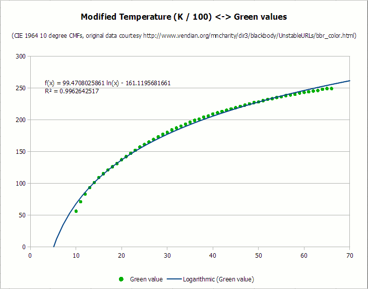
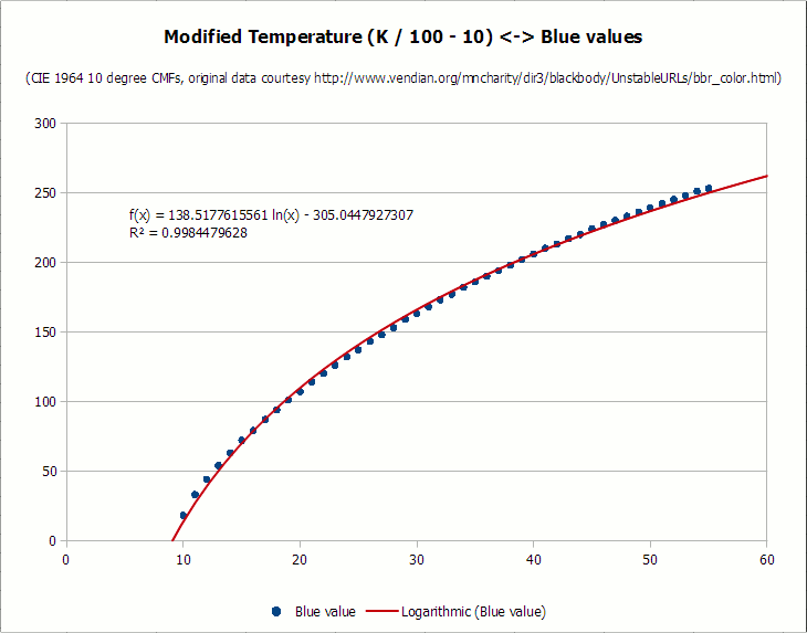
From this point on, I divided the data (without the “always 0” and “always 255” segments) into separate color components. In an ideal world, the curve can be adjusted to each set of points, but, unfortunately, in reality it is not so simple. Since the graph has a strong discrepancy between X and Y values ​​— all x values ​​are greater than 1000 and are displayed in 100 point segments, while y values ​​are between 255 and 0 — you had to transpose x data to get a better fit. In order to optimize, I first divided the value of x (temperature) by 100 for each color, and then subtracted as much as needed, if it significantly helped in fitting to the graph. Here are the resulting charts for each curve, as well as the most appropriate curve and the corresponding value of the coefficient of determination (R-square):









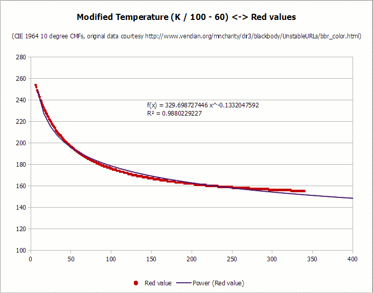
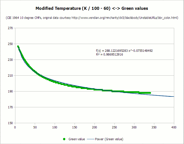
I apologize for the terrible kerning of fonts and hinting on diagrams. LibreOffice has a lot of advantages, but the inability to smooth fonts on graphics is completely shameful. I also do not like to extract diagrams from screenshots, because they do not have the export option, but it is better to leave it for later.

As you can see, all the curves are fairly well aligned, with the values ​​of the coefficient of determination above 0.987. I could spend more time fitting the curves, but this is enough for processing photos. No average person would say that the curves do not exactly correspond to the original idealized black body observations, right?

Algorithm

Here is the algorithm in all its glory.

First, the pseudocode:

     -  1000  40000. (   ,             40000 K).  ,             . Set Temperature = Temperature \ 100  : If Temperature <= 66 Then Red = 255 Else Red = Temperature - 60 Red = 329.698727446 * (Red ^ -0.1332047592) If Red < 0 Then Red = 0 If Red > 255 Then Red = 255 End If  : If Temperature <= 66 Then Green = Temperature Green = 99.4708025861 * Ln(Green) - 161.1195681661 If Green < 0 Then Green = 0 If Green > 255 Then Green = 255 Else Green = Temperature - 60 Green = 288.1221695283 * (Green ^ -0.0755148492) If Green < 0 Then Green = 0 If Green > 255 Then Green = 255 End If  : If Temperature >= 66 Then Blue = 255 Else If Temperature <= 19 Then Blue = 0 Else Blue = Temperature - 10 Blue = 138.5177312231 * Ln(Blue) - 305.0447927307 If Blue < 0 Then Blue = 0 If Blue > 255 Then Blue = 255 End If End If 

Please note that in the above pseudocode, Ln () means the natural logarithm . Also note that you can omit the “if the color is less than 0” checks, if the temperatures are always in the recommended range. (However, you still need to leave the check "if the color is more than 255").

As for the actual code, here is the exact Visual Basic function that I use in PhotoDemon . It is not yet optimized (for example, logarithms are much faster with correspondence tables), but at least the code is short and readable:

 '   ( )  RGB- Private Sub getRGBfromTemperature(ByRef r As Long, ByRef g As Long, ByRef b As Long, ByVal tmpKelvin As Long) Static tmpCalc As Double '      1000  40000  If tmpKelvin < 1000 Then tmpKelvin = 1000 If tmpKelvin > 40000 Then tmpKelvin = 40000 '   tmpKelvin \ 100,       tmpKelvin = tmpKelvin \ 100 '     '  If tmpKelvin <= 66 Then r = 255 Else ':  R-    0,988 tmpCalc = tmpKelvin - 60 tmpCalc = 329.698727446 * (tmpCalc ^ -0.1332047592) r = tmpCalc If r < 0 Then r = 0 If r > 255 Then r = 255 End If '  If tmpKelvin <= 66 Then ':  R-    0,996 tmpCalc = tmpKelvin tmpCalc = 99.4708025861 * Log(tmpCalc) - 161.1195681661 g = tmpCalc If g < 0 Then g = 0 If g > 255 Then g = 255 Else ':  R-    0,987 tmpCalc = tmpKelvin - 60 tmpCalc = 288.1221695283 * (tmpCalc ^ -0.0755148492) g = tmpCalc If g < 0 Then g = 0 If g > 255 Then g = 255 End If ',  If tmpKelvin >= 66 Then b = 255 ElseIf tmpKelvin <= 19 Then b = 0 Else ':  R-    0,998 tmpCalc = tmpKelvin - 10 tmpCalc = 138.5177312231 * Log(tmpCalc) - 305.0447927307 b = tmpCalc If b < 0 Then b = 0 If b > 255 Then b = 255 End If End Sub 

The function was used to generate a sample issue at the beginning of this article, so I can guarantee that it works.

Sample Images

Here's a great example of what color temperature adjustments can do. The image below — a poster for the HBO series “Real Blood” — spectacularly demonstrates the potential of adjusting color temperature. On the left - the original frame; on the right - adjusting the color temperature using the code above. With one click of the night scene can be remade for daylight.


Adjusting the color temperature in action

The real color temperature tool in my PhotoDemon program looks like this:


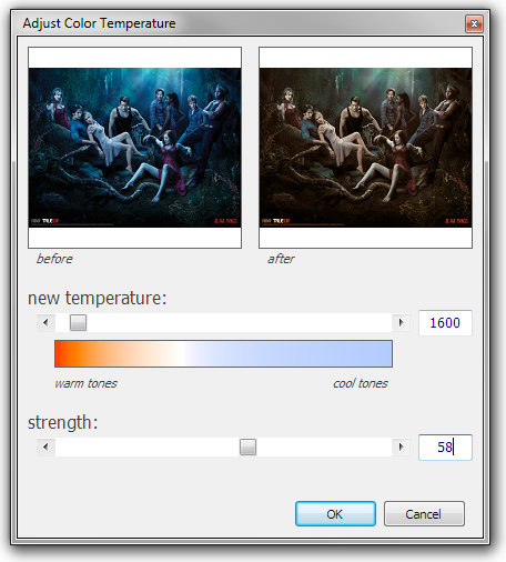
PhotoDemon Color Temperature Tool

Download the program and watch it in action.

Supplement, October 2014

Renault Bedar made a great online demo for this algorithm. Thank you, Reno!

Addition, April 2015

Thanks to everyone who suggested improvements to the original algorithm. I know that the article has a lot of comments, but they are worth reading if you plan to implement your own version.

I want to highlight two specific improvements. First, Neil B has kindly provided the best version for the original curve fitting functions, which slightly changes the temperature coefficients. The changes are described in detail in his excellent article .

Then Francis Lough added some comments and sample images that are very useful if you want to apply these transformations to photos. Its modifications produce a much more detailed image, as can be seen in the examples .