From the translator: exactly 175 years and 3 days ago quaternions were invented. In honor of this round date, I decided to choose a material that explains this concept in an understandable language.

The quaternion concept was invented by the Irish mathematician Sir William Rowan Hamilton on Monday October 16, 1843 in Dublin, Ireland. Hamilton and his wife went to the Irish Royal Academy , and going over the Royal Canal along the Broome Bridge , he made an amazing discovery, which he immediately scrawled on the stone of the bridge.

$$ $$i ^ 2 = j ^ 2 = k ^ 2 = ijk = -1$$

')

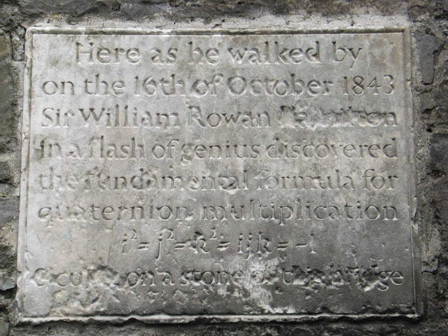
Memorial plaque on Broome Bridge over the Royal Canal in honor of the discovery of the fundamental multiplication formula for quaternions.

In this article I will try to explain the concept of quaternions in a simple to understand way. I will explain how you can visualize quaternion, and also talk about the different operations that can be performed with quaternions. In addition, I will compare the use of matrices, Euler angles and quaternions, and then try to explain when it is worth using quaternions instead of Euler angles or matrices, and when this is not necessary.

Content

• 1. Introduction
• 2. Complex numbers
  • 2.1. Addition and subtraction of complex numbers
  • 2.2. Multiply a complex number by a scalar value
  • 2.3. The product of complex numbers
  • 2.4. Square of complex numbers
  • 2.5. Conjugate complex numbers
  • 2.6. Absolute value of a complex number
  • 2.7. The quotient of two complex numbers
• 3. Degrees $$$i$
• 4. Complex plane
  
  • 4.1. Rotors
• 5. Quaternions
  • 5.1. Quaternions as an ordered pair
  • 5.2. Addition and subtraction of quaternions
  • 5.3. Quaternion product
  • 5.4. Real Quaternion
  • 5.5. Quaternion multiplication by scalar
  • 5.6. Pure Quaternions
  • 5.7. Additive Quaternion Form
  • 5.8. Unit quaternion
  • 5.9. Binary quaternion form
  • 5.10. Conjugate Quaternions
  • 5.11. Quaternion norm
  • 5.12. Normalization of Quaternion
  • 5.13. Reverse Quaternion
  • 5.14. Scalar product of quaternions
• 6. Turns
• 7. Interpolation of Quaternions
  
  • 7.1. SLERP
    
    • 7.1.1. Quaternion Difference
    • 7.1.2. Raising a quaternion to a power
    • 7.1.3. Fractional Quaternion Difference
    • 7.1.4. Factors to Consider
  • 7.2. SQUAD
• 8. Conclusion
• 9. Download demo
• 10. Reference materials

It is impossible to fully understand quaternions in 45 minutes.

There is a lot of math in this article, so it’s not for wimps.

Introduction

In computer graphics, matrices are used to describe the position in space (movement) as well as orientation in space (rotation). You can also use a single transformation matrix to describe the scale of the object. This matrix can be considered the “basis space”. If we multiply a vector or a point (or even another matrix) by a transformation matrix, then we “transform” this vector, point or matrix into the space represented by this matrix.

In this article I will not talk in detail about the transformation matrices. Details on transformation matrices can be found in my article Matrices .

In this article I want to talk about an alternative way to describe the orientation of an object (rotation) in space using quaternions.

Complex numbers

In order to fully understand the quaternions, we first need to understand where they came from. The quaternion principle is based on the concept of a system of complex numbers.

Along with the well-known sets of numbers ( natural , integer , real and rational ), the system of complex numbers adds a new set of numbers, called imaginary numbers. Imaginary numbers were invented to solve certain equations that had no solutions, for example:

$$ $$x ^ 2 + 1 = 0$$

To solve this expression, we need to declare that $$$x ^ 2 = -1$ , and this, as is known, is impossible, because the square of any number (positive or negative) is always positive.

Mathematicians could not accept the fact that the expression has no solution, so a new concept was invented - an imaginary number that can be used to solve such equations.

The imaginary number is as follows:

$$ $$i ^ 2 = -1$$

Do not try to understand this assumption, because there are no logical reasons for its existence. We just need to accept that $$$i$ - it's just some value, the square of which is equal $$$-1$ .

The set of imaginary numbers can be denoted as $$$\ mathbb {I}$ .

The set of complex numbers (denoted by the symbol $$$\ mathbb {C}$ Is the sum of the real and imaginary numbers in the following form:

$$ $$z = a + bi ~ a, b \ in \ mathbb {R}, ~~ i ^ 2 = -1$$

It can also be stated that all real numbers are complex with $$$b = 0$ , and all imaginary numbers are complex with $$$a = 0$ .

Addition and subtraction of complex numbers

Complex numbers can be added and subtracted by adding and subtracting real and imaginary parts.

Addition:

$$ $$(a_1 + b_1i) + (a_2 + b_2i) = (a_1 + a_2) + (b_1 + b_2) i$$

Subtraction:

$$ $$(a_1 + b_1i) - (a_2 + b_2i) = (a_1-a_2) + (b_1-b_2) i$$

Multiply a complex number by a scalar value

The complex number is multiplied by the scalar by multiplying each member of the complex number by the scalar:

$$ $$\ lambda (a + bi) = \ lambda {a} + \ lambda {b} i$$

The product of complex numbers

In addition, complex numbers can also be multiplied using ordinary algebraic rules.

$$ $$\ begin {array} {rcl} z_1 & = & (a_1 + b_1i) \\ z_2 & = & (a_2 + b_2i) \\ z_1z_2 & = & (a_1 + b_1i) (a_2 + b_2i) \\ & = & a_1a_2 + a_1b_2i + b_1a_2i + b_1b_2i ^ 2 \\ & = & (a_1a_2-b_1b_2) + (a_1b_2 + b_1a_2) i \ end {array}$$

Square of complex numbers

Also, a complex number can be squared by multiplying by itself:

$$ $$\ begin {array} {rcl} z & = & (a + bi) \\ z ^ 2 & = & (a + bi) (a + bi) \\ & = & (a ^ 2-b ^ 2) + 2abi \ end {array}$$

Conjugate complex numbers

The conjugate value of a complex number is a complex number with a modified sign of the imaginary part, denoted as $$$\ bar {z}$ or how $$$z ^ *$ .

$$ $$\ begin {array} {rcl} z & = & (a + bi) \\ z ^ * & = & (a-bi) \ end {array}$$

The multiplication of a complex number with its conjugate value gives an interesting result.

$$ $$\ begin {array} {rcl} z & = & (a + bi) \\ z ^ * & = & (a-bi) \\ zz ^ * & = & (a + bi) (a-bi) \ \ & = & a ^ 2-abi + abi + b ^ 2 \\ & = & a ^ 2 + b ^ 2 \ end {array}$$

Absolute value of a complex number

We can use the adjoint number of a complex number to calculate the absolute value (or rate , or value ) of a complex number. The absolute value of a complex number is the square root of a complex number multiplied by its conjugate number . It is denoted as $$$| z |$ :

$$ $$\ begin {array} {rcl} z & = & (a + bi) \\ | z | & = & \ sqrt {zz ^ *} \\ & = & \ sqrt {(a + bi) (a-bi)} \\ & = & \ sqrt {a ^ 2 + b ^ 2} \ end {array}$$

The quotient of two complex numbers

To calculate the quotient of two complex numbers, we multiply the numerator and denominator by the conjugate number of the denominator.

$$ $$\ begin {array} {rcl} z_1 & = & (a_1 + b_1i) \\ z_2 & = & (a_2 + b_2i) \\ \ cfrac {z_1} {z_2} & = & \ cfrac {a_1 + b_1i} { a_2 + b_2i} | ^ 2} {a_2 ^ 2 + b_2 ^ 2} \\ & = & \ cfrac {a_1a_2 + b_1b_2} {a_2 ^ 2 + b_2 ^ 2} + \ cfrac {b_1a_2-a_1b_2} {a_2 ^ 2 + b_2 ^ 2} i \ end {array}$$

Degrees $$$i$

If we claim that $$$i ^ 2 = -1$ then it must be possible to erect $$$i$ and to other degrees.

$$ $$\ begin {array} {rrrrrrr} i ^ 0 & = & & & & & 1 \\ i ^ 1 & = & & & & & i \\ i ^ 2 & = & & & & & -1 \\ i ^ 3 & = & ii ^ 2 & = & & & & i \\ i ^ 4 & = & i ^ {2} i ^ {2} & = & & & 1 \\ i ^ 5 & = & ii ^ 4 & = & & & i \\ i ^ 6 & = & ii ^ 5 & = & i ^ 2 & = & -1 \ end {array}$$

If we continue to record this series, we notice the pattern $$$(1, i, -1, -i, 1, \ dots)$ .

A similar pattern occurs with increasing negative degrees.

$$ $$\ begin {array} {rcr} i ^ 0 & = & 1 \\ i ^ {- 1} & = & -i \\ i ^ {- 2} & = & -1 \\ i ^ {- 3} & = & i \\ i ^ {- 4} & = & 1 \\ i ^ {- 5} & = & -i \\ i ^ {- 6} & = & -1 \ end {array}$$

You may have seen this pattern in math, but in the form $$$(x, y, -x, -y, x, \ dots)$ which is obtained by rotating the point 90 ° counterclockwise on a two-dimensional Cartesian plane; row $$$(x, -y, -x, y, x, \ dots)$ created by turning a point 90 ° degrees on a two-dimensional Cartesian plane.


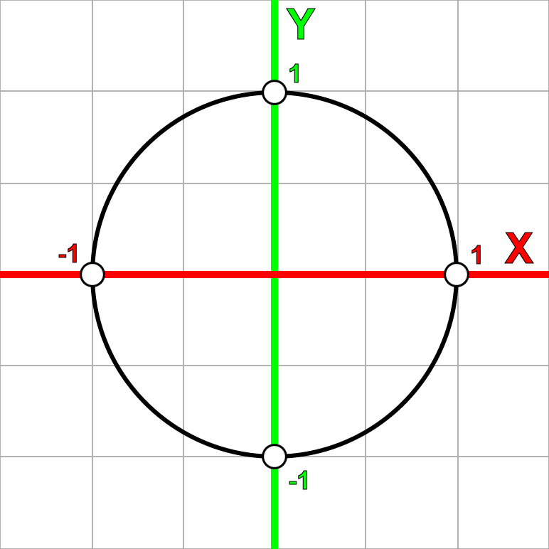
Cartesian plane

Complex plane

We can similarly apply complex numbers to a two-dimensional grid, called the complex plane , by tying the real part to the horizontal axis, and the imaginary part to the vertical one.


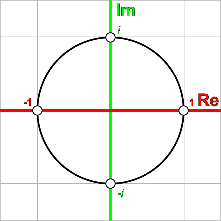
Complex plane

As can be seen from the previous row, we can say that if we multiply the complex number by $$$i$ then we can rotate the complex number on the complex plane with a step of 90 °.

Let's check if this is true. We take an arbitrary point on the complex plane. $$$p$ :

$$ $$p = 2 + i$$

and multiply it by $$$i$ by receiving $$$q$ :

$$ $$\ begin {array} {rcl} p & = & 2 + i \\ q & = & pi \\ & = & (2 + i) i \\ & = & 2i + i ^ 2 \\ & = & - 1 + 2i \ end {array}$$

Multiplying $$$q$ on $$$i$ get $$$r$ :

$$ $$\ begin {array} {rcl} q & = & -1 + 2i \\ r & = & qi \\ & = & (-1 + 2i) i \\ & = & -i + 2i ^ 2 \\ & = & -2-i \ end {array}$$

And multiplying $$$r$ on $$$i$ get $$$s$ :

$$ $$\ begin {array} {rcl} r & = & -2-i \\ s & = & ri \\ & = & (-2-i) i \\ & = & -2i-i ^ 2 \\ & = & 1-2i \ end {array}$$

And multiplying $$$s$ on $$$i$ get $$$t$ :

$$ $$\ begin {array} {rcl} s & = & 1-2i \\ t & = & si \\ & = & (1-2i) i \\ & = & i-2i ^ 2 \\ & = & 2 + i \ end {array}$$

And we got exactly what we started from ( $$$p$ ). If we put these complex numbers on the complex plane, we get the following result.


Complex numbers on a complex plane

Now we can rotate on the complex plane and clockwise, multiplying the complex number by $$$-i$ .

Rotors

We can also perform arbitrary turns on the complex plane by specifying a complex number in the following form:

$$ $$q = \ cos \ theta + i \ sin \ theta$$

When multiplying any complex number by rotor $$$q$ we get the general formula:

$$ $$\ begin {array} {rcl} p & = & a + bi \ q & = & \ cos \ theta + i \ sin \ theta \\ pq & = & (a + bi) (\ cos \ theta + i \ sin \ theta) \\ a ^ {\ prime} + b ^ {\ prime} i & = & a \ cos \ theta-b \ sin \ theta + (a \ sin \ theta + b \ cos \ theta) i \ end {array}$$

What can also be written in matrix form:

$$ $$\ begin {bmatrix} a ^ {\ prime} & -b ^ {\ prime} \\ b ^ {\ prime} & a ^ {\ prime} \ end {bmatrix} = \ begin {bmatrix} \ cos \ theta & - \ sin \ theta \\ \ sin \ theta & \ cos \ theta \ end {bmatrix} \ begin {bmatrix} a & -b \\ b & a \ end {bmatrix}$$

What is the way to turn counterclockwise of an arbitrary point on the complex plane relative to the point of origin of coordinates.

Quaternions

Having learned about the system of complex numbers and the complex plane, we can derive them into three-dimensional space, adding to the system of numbers along with $$$i$ two more imaginary numbers.

Quaternions have the following generalized form.

$$ $$q = s + xi + yj + zk ~, s, x, y, z \ in \ mathbb {R}$$

Where according to Hamilton's famous expression:

$$ $$i ^ 2 = j ^ 2 = k ^ 2 = ijk = -1$$

$$ $$\ begin {array} {ccc} ij = k & jk = i & ki = j \\ ji = -k & kj = -i & ik = -j \ end {array}$$

You may notice that the relationship between $$$i$ , $$$j$ and $$$k$ very similar to the rules of vector multiplication of unitary cartesian vectors:

$$ $$\ begin {array} {ccc} \ mathbf {x} \ times \ mathbf {y} = \ mathbf {z} & \ mathbf {y} \ times \ mathbf {z} = \ mathbf {x} & \ mathbf { z} \ times \ mathbf {x} = \ mathbf {y} \\ \ mathbf {y} \ times \ mathbf {x} = - \ mathbf {z} & \ mathbf {z} \ times \ mathbf {y} = - \ mathbf {x} & \ mathbf {x} \ times \ mathbf {z} = - \ mathbf {y} \ end {array}$$

Hamilton also noticed that imaginary numbers $$$i$ , $$$j$ and $$$k$ can be used to represent three Cartesian unit vectors $$$\ mathbf {i}$ , $$$\ mathbf {j}$ and $$$\ mathbf {k}$ with the same properties of imaginary numbers so that $$$\ mathbf {i} ^ 2 = \ mathbf {j} ^ 2 = \ mathbf {k} ^ 2 = -1$ .


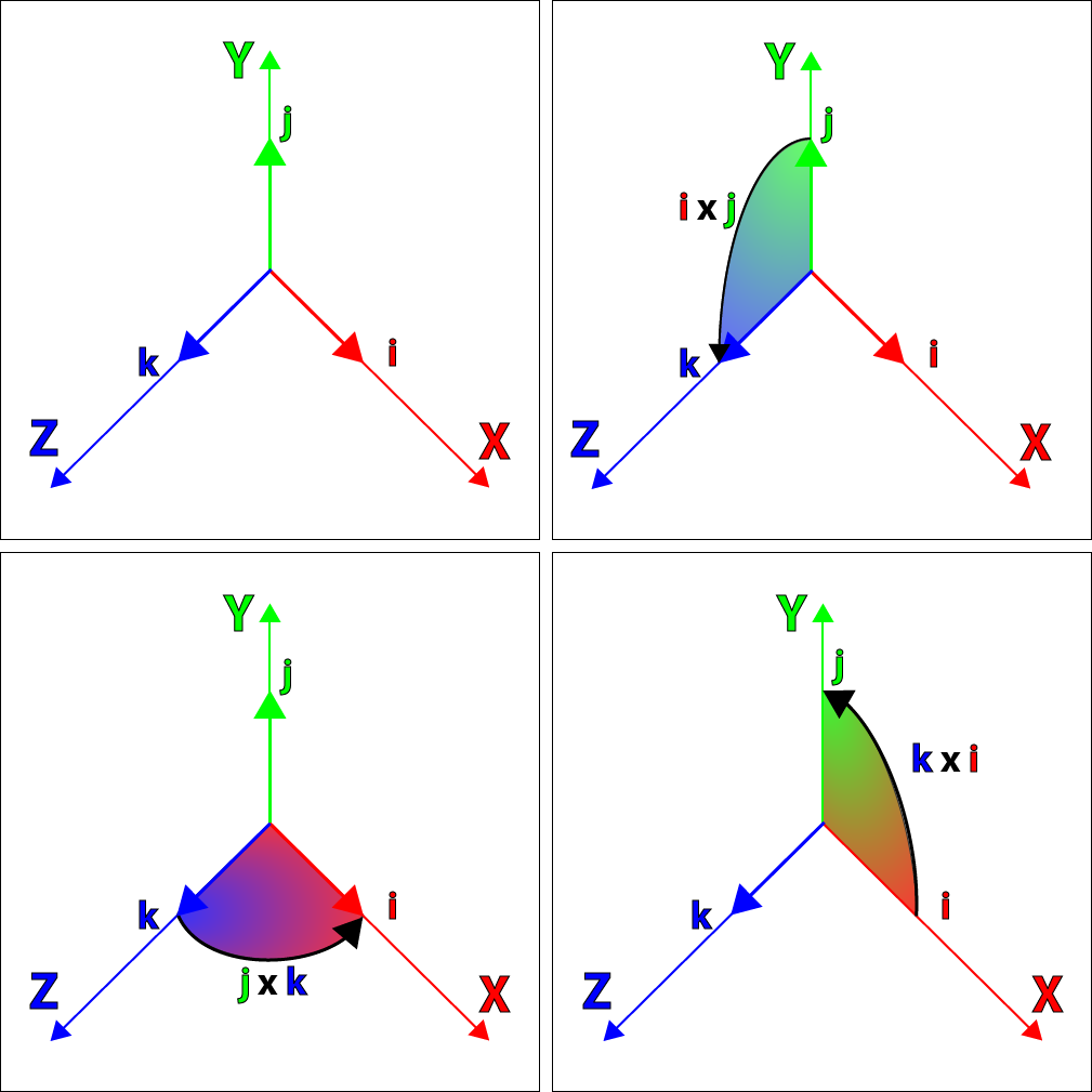
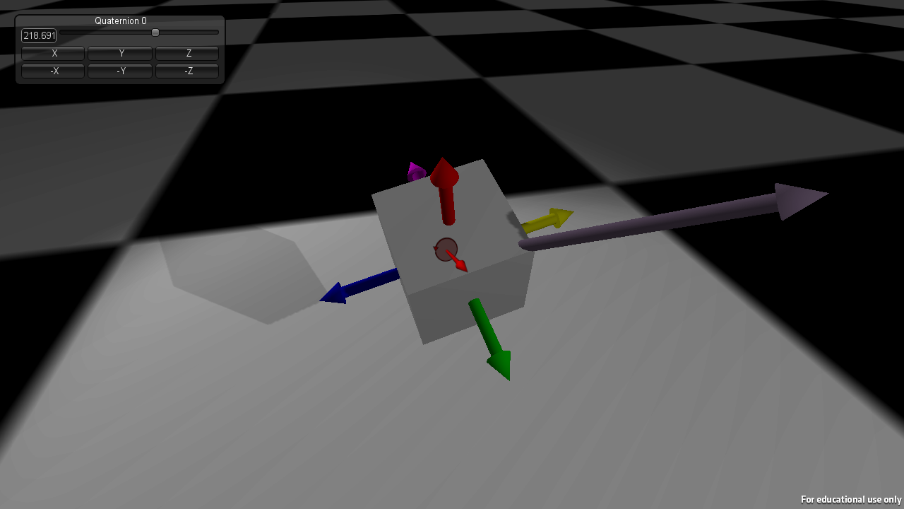
Graphic representation of properties $$$\ mathbf {ij}$ , $$$\ mathbf {jk}$ , $$$\ mathbf {ki}$

The above image graphically presents the relationships between Cartesian unit vectors in the form $$$\ mathbf {i}$ , $$$\ mathbf {j}$ and $$$\ mathbf {k}$ .

Quaternions as an ordered pair

We can also represent quaternions in the form of an ordered pair:

$$ $$q = [s, \ mathbf {v}] ~~ s \ in \ mathbb {R}, \ mathbf {v} \ in \ mathbb {R} ^ 3$$

Where $$$\ mathbf {v}$ can also be represented as its individual components:

$$ $$q = [s, x \ mathbf {i} + y \ mathbf {j} + z \ mathbf {k}] ~~ s, x, y, z \ in \ mathbb {R}$$

With this entry, we can more easily present the common features of quaternions and complex numbers.

Addition and subtraction of quaternions

Quaternions can be added and subtracted in the same way as complex numbers:

$$ $$\ begin {array} {rcl} q_a & = & [s_a, \ mathbf {a}] \\ q_b & = & [s_b, \ mathbf {b}] \\ q_a + q_b & = & [s_a + s_b, \ mathbf {a} + \ mathbf {b}] \\ q_a-q_b & = & [s_a-s_b, \ mathbf {a} - \ mathbf {b}] \ end {array}$$

Quaternion products

We can also express the product of two quaternions:

$$ $$\ begin {array} {rcl} q_a & = & [s_a, \ mathbf {a}] \\ q_b & = & [s_b, \ mathbf {b}] \\ q_ {a} q_ {b} & = & [s_ {a}, \ mathbf {a}] [s_ {b}, \ mathbf {b}] \\ & = & (s_ {a} + x_ {a} i + y_ {a} j + z_ {a } k) (s_ {b} + x_ {b} i + y_ {b} j + z_ {b} k) \\ & = & (s_ {a} s_ {b} -x_ {a} x_ {b} -y_ {a} y_ {b} -z_ {a} z_ {b}) \\ & & + (s_ {a} x_ {b} + s_ {b} x {a} + y_ {a} z_ {b } -y_ {b} z_ {a}) i \\ & & + (s_ {a} y_ {b} + s_ {b} y_ {a} + z_ {a} x_ {b} -z_ {b} x_ {a}) j \\ & & + (s_ {a} z_ {b} + s_ {b} z_ {a} + x_ {a} y_ {b} -x_ {b} y_ {a}) k \ end {array}$$

What gives us another quaternion. If we replace the imaginary numbers in the previous expression $$$i$ , $$$j$ and $$$k$ ordered pairs (also known as quaternion units), we obtain

$$ $$i = [0, \ mathbf {i}] ~ j = [0, \ mathbf {j}] ~ k = [0, \ mathbf {k}]$$

And substituting back into the original expression with $$$[1, \ mathbf {0}] = 1$ , we get:

$$ $$\ begin {array} {rcl} [s_ {a}, \ mathbf {a}] [s_ {b}, \ mathbf {b}] & = & (s_ {a} s_ {b} -x_ {a} x_ {b} -y_ {a} y_ {b} -z_ {a} z_ {b}) [1, \ mathbf {0}] \\ & & + (s_ {a} x_ {b} + s_ {b } x {a} + y_ {a} z_ {b} -y_ {b} z_ {a}) [0, \ mathbf {i}] \\ & & + (s_ {a} y_ {b} + s_ { b} y_ {a} + z_ {a} x_ {b} -z_ {b} x_ {a}) [0, \ mathbf {j}] \\ & & + (s_ {a} z_ {b} + s_ {b} z_ {a} + x_ {a} y_ {b} -x_ {b} y_ {a}) [0, \ mathbf {k}] \ end {array}$$

Expanding this expression into the sum of ordered pairs, we get:

$$ $$\ begin {array} {rcl} [s_ {a}, \ mathbf {a}] [s_ {b}, \ mathbf {b}] & = & [s_ {a} s_ {b} -x_ {a} x_ {b} -y_ {a} y_ {b} -z_ {a} z_ {b}, \ mathbf {0}] \\ & & + [0, (s_ {a} x_ {b} + s_ {b } x {a} + y_ {a} z_ {b} -y_ {b} z_ {a}) \ mathbf {i}] \\ & & + [0, (s_ {a} y_ {b} + s_ { b} y_ {a} + z_ {a} x_ {b} -z_ {b} x_ {a}) \ mathbf {j}] \\ & & + [0, (s_ {a} z_ {b} + s_ {b} z_ {a} + x_ {a} y_ {b} -x_ {b} y_ {a}) \ mathbf {k}] \ end {array}$$

If you multiply by a quaternion unit and extract the common vector components, you can rewrite this equation as follows:

$$ $$\ begin {array} {rcl} [s_ {a}, \ mathbf {a}] [s_ {b}, \ mathbf {b}] & = & [s_ {a} s_ {b} -x_ {a} x_ {b} -y_ {a} y_ {b} -z_ {a} z_ {b}, \ mathbf {0}] \\ & & + [0, s_ {a} (x_ {b} \ mathbf {i } + y_ {b} \ mathbf {j} + z_ {b} \ mathbf {k}) + s_ {b} (x_ {a} \ mathbf {i} + y_ {a} \ mathbf {j} + z_ { a} \ mathbf {k}) \\ & & + (y_ {a} z_ {b} -y_ {b} z_ {a}) \ mathbf {i} + (z_ {a} x_ {b} -z_ { b} x_ {a}) \ mathbf {j} + (x_ {a} y_ {b} -x_ {b} y_ {a}) \ mathbf {k}] \ end {array}$$

This equation gives us the sum of two ordered pairs. The first ordered pair is a real quaternion , and the second is a pure quaternion. These two ordered pairs can be combined into one ordered pair:

$$ $$\ begin {array} {rcl} [s_ {a}, \ mathbf {a}] [s_ {b}, \ mathbf {b}] & = & [s_ {a} s_ {b} -x_ {a} x_ {b} -y_ {a} y_ {b} -z_ {a} z_ {b}, \\ & & s_ {a} (x_ {b} \ mathbf {i} + y_ {b} \ mathbf {j } + z_ {b} \ mathbf {k}) + s_ {b} (x_ {a} \ mathbf {i} + y_ {a} \ mathbf {j} + z_ {a} \ mathbf {k}) \\ & & + (y_ {a} z_ {b} -y_ {b} z_ {a}) \ mathbf {i} + (z_ {a} x_ {b} -z_ {b} x_ {a}) \ mathbf { j} + (x_ {a} y_ {b} -x_ {b} y_ {a}) \ mathbf {k}] \ end {array}$$

If we substitute, we get

$$ $$\ begin {array} {rcl} \ mathbf {a} & = & x_ {a} \ mathbf {i} + y_ {a} \ mathbf {j} + z_ {a} \ mathbf {k} \\ \ mathbf {b} & = & x_ {b} \ mathbf {i} + y_ {b} \ mathbf {j} + z_ {b} \ mathbf {k} \\ \ mathbf {a} \ cdot \ mathbf {b} & = & x_ {a} x_ {b} + y_ {a} y_ {b} + z_ {a} z_ {b} \\ \ mathbf {a} \ times \ mathbf {b} & = & (y_ {a} z_ {b} -y_ {b} z_ {a}) \ mathbf {i} + (z_ {a} x_ {b} -z_ {b} x_ {a}) \ mathbf {j} + (x_ {a} y_ {b} -x_ {b} y_ {a}) \ mathbf {k} \ end {array}$$

We get:

$$ $$[s_ {a}, \ mathbf {a}] [s_ {b}, \ mathbf {b}] = [s_ {a} s_ {b} - \ mathbf {a} \ cdot \ mathbf {b}, s_ {a} \ mathbf {b} + s_ {b} \ mathbf {a} + \ mathbf {a} \ times \ mathbf {b}]$$

This is the general equation of the product of quaternions.

Real Quaternion

A real quaternion is a quaternion that includes a vector $$$\ mathbf {0}$ :

$$ $$q = [s, \ mathbf {0}]$$

And the product of two real quaternions is another real quaternion:

$$ $$\ begin {array} {rcl} q_a & = & [s_a, \ mathbf {0}] \\ q_b & = & [s_b, \ mathbf {0}] \\ q_ {a} q_ {b} & = & [s_a, \ mathbf {0}] [s_b, \ mathbf {0}] \\ & = & [s_ {a} s_ {b}, \ mathbf {0}] \ end {array}$$

Which is similar to the product of two complex numbers containing a zero imaginary term.

$$ $$\ begin {array} {rcl} z_1 & = & a_1 + 0i \\ z_2 & = & a_2 + 0i \\ z_ {1} z_ {2} & = & (a_1 + 0i) (a_2 + 0i) \\ & = & a_ {1} a_ {2} \ end {array}$$

Quaternion multiplication by scalar

We can also multiply the quaternion by a scalar, while adhering to the following rule:

$$ $$\ begin {array} {rcl} q & = & [s, \ mathbf {v}] \\ \ lambda {q} & = & \ lambda [s, \ mathbf {v}] \\ & = & [\ lambda {s}, \ lambda \ mathbf {v}] \ end {array}$$

We can verify this with the help of the above product of real quaternions, by multiplying the quaternion by a scalar as a real quaternion:

$$ $$\ begin {array} {rcl} q & = & [s, \ mathbf {v}] \\ \ lambda & = & [\ lambda, \ mathbf {0}] \\ \ lambda {q} & = & [ \ lambda, \ mathbf {0}] [s, \ mathbf {v}] \\ & = & [\ lambda {s}, \ lambda \ mathbf {v}] \ end {array}$$

Pure Quaternions

In addition to real quaternions, Hamilton also defined a pure quaternion as a quaternion with a zero scalar member:

$$ $$q = [0, \ mathbf {v}]$$

Or if you write down the components:

$$ $$q = xi + yj + zk$$

And again we can take the product of two pure quaternions:

$$ $$\ begin {array} {rcl} q_a & = & [0, \ mathbf {a}] \\ q_b & = & [0, \ mathbf {b}] \\ q_ {a} q_ {b} & = & [0, \ mathbf {a}] [0, \ mathbf {b}] \\ & = & [- \ mathbf {a} \ cdot \ mathbf {b}, \ mathbf {a} \ times \ mathbf {b} ] \ end {array}$$

in accordance with the above rule of quaternion products.

Additive Quaternion Form

In addition, we can express quaternions as the sum of real and pure parts of a quaternion:

$$ $$\ begin {array} {rcl} q & = & [s, \ mathbf {v}] \\ & = & [s, \ mathbf {0}] + [0, \ mathbf {v}] \ end {array }$$

Unit quaternion

Taking an arbitrary vector $$$\ mathbf {v}$ , it is possible to express this vector both through its scalar value, and through its direction as follows:

$$ $$\ mathbf {v} = v \ mathbf {\ hat {v}} ~ \ text {where} ~ v = | \ mathbf {v} | ~ \ text {and} ~ | \ mathbf {\ hat {v}} | = 1$$

Combining this definition with the definition of a pure quaternion, we get:

$$ $$\ begin {array} {rcl} q & = & [0, \ mathbf {v}] \\ & = & [0, v \ mathbf {\ hat {v}}] \\ & = & v [0, \ mathbf {\ hat {v}}] \ end {array}$$

We can also describe a unit quaternion having a zero scalar and a unit vector:

$$ $$\ hat {q} = [0, \ mathbf {\ hat {v}}]$$

Binary quaternion form

Now we can combine the definitions of the single quaternion and the additive form of the quaternion, obtaining the form of quaternions, similar to the record used in the description of complex numbers:

$$ $$\ begin {array} {rcl} q & = & [s, \ mathbf {v}] \\ & = & [s, \ mathbf {0}] + [0, \ mathbf {v}] \\ & = & [s, \ mathbf {0}] + v [0, \ mathbf {\ hat {v}}] \\ & = & s + v \ hat {q} \ end {array}$$

This gives us a way to represent a quaternion in a form very similar to complex numbers:

$$ $$\ begin {array} {rcl} z & = & a + bi \\ q & = & s + v \ hat {q} \ end {array}$$

Quaternion Conjugate Number

The adjoint number of a quaternion can be calculated by taking the vector part of the quaternion opposite in sign:

$$ $$\ begin {array} {rcl} q & = & [s, \ mathbf {v}] \\ q ^ * & = & [s, - \ mathbf {v}] \ end {array}$$

The product of a quaternion and its conjugate number gives us the following:

$$ $$\ begin {array} {rcl} qq ^ * & = & [s, \ mathbf {v}] [s, - \ mathbf {v}] \\ & = & [s ^ 2- \ mathbf {v} \ cdot- \ mathbf {v}, - s \ mathbf {v} + s \ mathbf {v} + \ mathbf {v} \ times- \ mathbf {v}] \\ & = & [s ^ 2 + \ mathbf { v} \ cdot \ mathbf {v}, \ mathbf {0}] \\ & = & [s ^ 2 + v ^ 2, \ mathbf {0}] \ end {array}$$

Quaternion norm

Recall the definition of the norm of a complex number:

$$ $$\ begin {array} {rcl} | z | & = & \ sqrt {a ^ 2 + b ^ 2} \\ zz ^ * & = & | z | ^ 2 \ end {array}$$

Similarly, the rate (or value) of a quaternion is defined as:

$$ $$\ begin {array} {rcl} q & = & [s, \ mathbf {v}] \\ | q | & = & \ sqrt {s ^ 2 + v ^ 2} \ end {array}$$

This allows us to express the quaternion rate as follows:

$$ $$qq ^ * = | q | ^ 2$$

Normalization of Quaternion

Having a definition of the quaternion norm, we can use it to normalize the quaternion. Quaternion is normalized by dividing by $$$| q |$ :

$$ $$q ^ {\ prime} = \ frac {q} {\ sqrt {s ^ 2 + v ^ 2}}$$

For example, let's normalize the quaternion:

$$ $$q = [1,4 \ mathbf {i} +4 \ mathbf {j} -4 \ mathbf {k}]$$

First we need to calculate the quaternion rate :

$$ $$\ begin {array} {rcl} | q | & = & \ sqrt {1 ^ 2 + 4 ^ 2 + 4 ^ 2 + (- 4) ^ 2} \\ & = & \ sqrt {49} \\ & = & 7 \ end {array}$$

Then we must divide the quaternion by the quaternion norm to calculate the normalized quaternion:

$$ $$\ begin {array} {rcl} q ^ {\ prime} & = & \ cfrac {q} {| q |} \\ [1.0em] & = & \ cfrac {(1 + 4 \ mathbf {i} + 4 \ mathbf {j} -4 \ mathbf {k})} {7} \\ [1.0em] & = & \ cfrac {1} {7} + \ cfrac {4} {7} \ mathbf {i} + \ cfrac {4} {7} \ mathbf {j} - \ cfrac {4} {7} \ mathbf {k} \ end {array}$$

Reverse Quaternion

Reverse quaternion is denoted by $$$q ^ {- 1}$ . To calculate the inverse quaternion, we take the adjoint number of the quaternion and divide it by the square of the norm:

$$ $$q ^ {- 1} = \ frac {q ^ *} {| q | ^ 2}$$

To show this, we can use the definition of a reciprocal:

$$ $$qq ^ {- 1} = [1, \ mathbf {0}] = 1$$

And multiply both sides by the conjugate number of the quaternion, which will give us:

$$ $$q ^ {*} qq ^ {- 1} = q ^ {*}$$

By substitution we get:

$$ $$\ begin {array} {rcl} | q | ^ {2} q ^ {- 1} & = & q ^ {*} \\ q ^ {- 1} & = & \ cfrac {q ^ {*}} {| q | ^ {2}} \ end {array}$$

For single quaternions-norms whose norm is equal to 1, we can write:

$$ $$q ^ {- 1} = q ^ {*}$$

Scalar product of quaternions

Similarly to the scalar product of vectors, we can calculate the scalar product of two quaternions by multiplying the corresponding scalar parts and summing up the results:

$$ $$\ begin {array} {rcl} q_1 & = & [s_1, x_1 \ mathbf {i} + y_1 \ mathbf {j} + z_1 \ mathbf {k}] \\ q_2 & = & [s_2, x_2 \ mathbf { i} + y_2 \ mathbf {j} + z_2 \ mathbf {k}] \\ q_1 {\ cdot} q_2 & = & s_ {1} s_ {2} + x_ {1} x_ {2} + y_ {1} y_ {2} + z_ {1} z_ {2} \ end {array}$$

We can also use the scalar product of quaternions to calculate the angular difference between quaternions:

$$ $$\ cos \ theta = \ frac {s_ {1} s_ {2} + x_ {1} x_ {2} + y_ {1} y_ {2} + z_ {1} z_ {2}} {| q_ {1 } || q_ {2} |}$$

For unit quaternions-norms, we can simplify the equation:

$$ $$\ cos \ theta = s_ {1} s_ {2} + x_ {1} x_ {2} + y_ {1} y_ {2} + z_ {1} z_ {2}$$

Turns

Let me remind you that we have defined a special form of a complex number called a rotor , which can be used to rotate a point on a two-dimensional plane as follows:

$$ $$q = \ cos \ theta + i \ sin \ theta$$

Due to the similarity of complex numbers with quaternions, it should be possible to express a quaternion that can be used to rotate a point in three-dimensional space:

$$ $$q = [\ cos \ theta, \ sin \ theta \ mathbf {v}]$$

Let's check if this theory is correct by calculating the product of the quaternion $$$q$ and vectors $$$\ mathbf {p}$ . First, we can express $$$\ mathbf {p}$ as pure quaternion in the following form:

$$ $$p = [0, \ mathbf {p}]$$

BUT $$$q$ - is a single quaternion-norm in the form:

$$ $$q = [s, \ lambda \ mathbf {\ hat {v}}]$$

Then

$$ $$\ begin {array} {rcl} p ^ {\ prime} & = & qp \\ & = & [s, \ lambda \ mathbf {\ hat {v}}] [0, \ mathbf {p}] \\ & = & [- \ lambda \ mathbf {\ hat {v}} \ cdot \ mathbf {p}, s \ mathbf {p} + \ lambda \ mathbf {\ hat {v}} \ times \ mathbf {p}] \ end {array}$$

We see that the result is a common quaternion with scalar and vector parts.

Let's first consider the “special” case in which $$$\ mathbf {p}$ perpendicular $$$\ mathbf {\ hat {v}}$ . In this case, the scalar member $$$- \ lambda \ mathbf {\ hat {v}} \ cdot \ mathbf {p} = 0$ and the result becomes a pure quaternion:

$$ $$p ^ {\ prime} = [0, s \ mathbf {p} + \ lambda \ mathbf {\ hat {v}} \ times \ mathbf {p}]$$

In this case, to turn $$$\ mathbf {p}$ regarding $$$\ mathbf {\ hat {v}}$ we just substitute $$$s = \ cos \ theta$ and $$$\ lambda = \ sin \ theta$ .

$$ $$p ^ {\ prime} = [0, \ cos \ theta \ mathbf {p} + \ sin \ theta \ mathbf {\ hat {v}} \ times \ mathbf {p}]$$

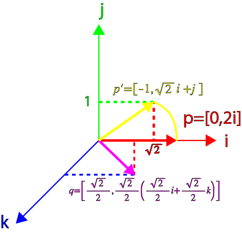
For example, let's rotate the vector $$$\ mathbf {p}$ 45 ° relative to the Z axis; then our quaternion $$$q$ will be equal to:

$$ $$\ begin {array} {rcl} q & = & [\ cos \ theta, \ sin \ theta \ mathbf {k}] \\ & = & \ left [\ frac {\ sqrt {2}} {2}, \ frac {\ sqrt {2}} {2} \ mathbf {k} \ right] \ end {array}$$

And let's take a vector $$$\ mathbf {p}$ which refers to a special case where $$$\ mathbf {p}$ perpendicular $$$\ mathbf {k}$ :

$$ $$p = [0,2 \ mathbf {i}]$$

Now let's find the piece

$$ $$qp$$

:

$$ $$\ begin {array} {rcl} p ^ {\ prime} & = & qp \\ & = & \ left [\ frac {\ sqrt {2}} {2}, \ frac {\ sqrt {2}} { 2} \ mathbf {k} \ right] [0,2 \ mathbf {i}] \\ & = & \ left [0,2 \ frac {\ sqrt {2}} {2} \ mathbf {i} +2 \ frac {\ sqrt {2}} {2} \ mathbf {k} \ times \ mathbf {i} \ right] \\ & = & [0, \ sqrt {2} \ mathbf {i} + \ sqrt {2 } \ mathbf {j}] \ end {array}$$

What gives us a pure quaternion, rotated 45 ° relative to the axis $$$\ mathbf {k}$ . We can also make sure that the value of the final vector is preserved:

$$ $$\ begin {array} {rcl} | \ mathbf {p} ^ {\ prime} | & = & \ sqrt {\ sqrt {2} ^ {2} + \ sqrt {2} ^ {2}} \\ & = & 2 \ end {array}$$

Exactly what we expected!

We can show it graphically with the following image:


Quaternion rotation (1)

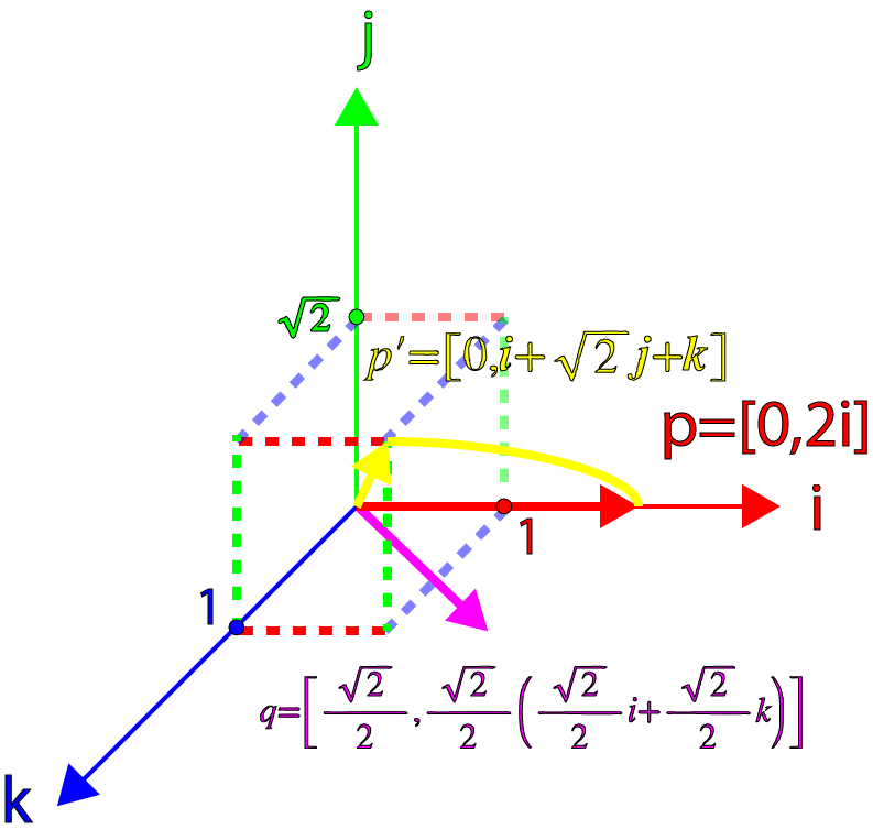
Now let's consider a quaternion that is not orthogonal to $$$\ mathbf {p}$ . If we take for the vector part of the quaternion an offset of 45 ° from $$$\ mathbf {p}$ , we get:

$$ $$\ begin {array} {rcl} \ mathbf {\ hat {v}} & = & \ frac {\ sqrt {2}} {2} \ mathbf {i} + \ frac {\ sqrt {2}} {2 } \ mathbf {k} \\ \ mathbf {p} & = & 2 \ mathbf {i} \\ q & = & [\ cos \ theta, \ sin \ theta \ mathbf {\ hat {v}}] \\ p & = & [0, \ mathbf {p}] \ end {array}$$

And multiplying our vector $$$\ mathbf {p}$ on $$$q$ , we get:

$$ $$\ begin {array} {rcl} p ^ {\ prime} & = & qp \\ & = & [\ cos \ theta, sin \ theta \ mathbf {\ hat {v}}] [0, \ mathbf {p }] \\ & = & [- \ sin \ theta \ mathbf {\ hat {v}} \ cdot \ mathbf {p}, \ cos \ theta \ mathbf {p} + \ sin \ theta \ mathbf {\ hat { v}} \ times \ mathbf {p}] \ end {array}$$

After substitution $$$\ mathbf {\ hat {v}}$ , $$$\ mathbf {p}$ and $$$\ theta = 45 ^ {\ circ}$ we get:

$$ $$\ begin {array} {rcl} p ^ {\ prime} & = & \ left [- \ frac {\ sqrt {2}} {2} \ left (\ frac {\ sqrt {2}} {2} \ mathbf {i} + \ frac {\ sqrt {2}} {2} \ mathbf {k} \ right) \ cdot (2 \ mathbf {i}), \ frac {\ sqrt {2}} {2} 2 \ mathbf {i} + \ frac {\ sqrt {2}} {2} \ left (\ frac {\ sqrt {2}} {2} \ mathbf {i} + \ frac {\ sqrt {2}} {2} \ mathbf {k} \ right) \ times2 \ mathbf {i} \ right] \\ & = & [-1, \ sqrt {2} \ mathbf {i} + \ mathbf {j}] \ end {array}$$

That is, it is no longer a pure quaternion, it is not rotated by 45 °, and the vector norm is no longer equal to 2 (it decreased to $$$\ sqrt {3}$ ).

This result can be shown graphically.


Quaternion rotation (2)

Strictly speaking, it is incorrect to represent a quaternion. $$$p ^ {\ prime}$ in three-dimensional space, because in fact it is a four-dimensional vector! For the sake of simplification, I will show only the vector component of quaternions.

However, all is not lost. Hamilton found out (but did not publish this) that if we then multiply the result $$$qp$ the opposite of $$$q$ , the result is a pure quaternion, and the norm of the vector component is preserved. Let's see if we can apply this in our example.

First, let's calculate $$$q ^ {- 1}$ :

$$ $$\ begin {array} {rcl} q & = & \ left [\ cos \ theta, \ sin \ theta \ left (\ frac {\ sqrt {2}} {2} \ mathbf {i} + \ frac {\ sqrt {2}} {2} \ mathbf {k} \ right) \ right] \\ q ^ {- 1} & = & \ left [\ cos \ theta, - \ sin \ theta \ left (\ frac {\ sqrt {2}} {2} \ mathbf {i} + \ frac {\ sqrt {2}} {2} \ mathbf {k} \ right) \ right] \ end {array}$$

With $$$\ theta = 45 ^ {\ circ}$ we get:

$$ $$\ begin {array} {rcl} q ^ {- 1} & = & \ left [\ frac {\ sqrt {2}} {2}, - \ frac {\ sqrt {2}} {2} \ left ( \ frac {\ sqrt {2}} {2} \ mathbf {i} + \ frac {\ sqrt {2}} {2} \ mathbf {k} \ right) \ right] \\ & = & \ frac {1 } {2} \ left [\ sqrt {2}, - \ mathbf {i} - \ mathbf {k} \ right] \ end {array}$$

Combining the previous value $$$qp$ and $$$q ^ {- 1}$ , we get:

$$ $$\ begin {array} {rcl} qp & = & \ left [-1, \ sqrt {2} \ mathbf {i} + \ mathbf {j} \ right] \\ qpq ^ {- 1} & = & \ left [-1, \ sqrt {2} \ mathbf {i} + \ mathbf {j} \ right] \ frac {1} {2} \ left [\ sqrt {2}, - \ mathbf {i} - \ mathbf {k} \ right] \\ & = & \ frac {1} {2} \ left [- \ sqrt {2} - \ left (\ sqrt {2} \ mathbf {i} + \ mathbf {j} \ right ) \ cdot (- \ mathbf {i} - \ mathbf {k}), \ mathbf {i} + \ mathbf {k} + \ sqrt {2} \ left (\ sqrt {2} \ mathbf {i} + \ mathbf {j} \ right) - \ mathbf {i} + \ sqrt {2} \ mathbf {j} + \ mathbf {k} \ right] \\ & = & \ frac {1} {2} \ left [- \ sqrt {2} + \ sqrt {2}, \ mathbf {i} + \ mathbf {k} +2 \ mathbf {i} + \ sqrt {2} \ mathbf {j} - \ mathbf {i} + \ sqrt {2} \ mathbf {j} + \ mathbf {k} \ right] \\ & = & \ left [0, \ mathbf {i} + \ sqrt {2} \ mathbf {j} + \ mathbf {k} \ right] \ end {array}$$

What is a pure quaternion, and the norm of the result is:

$$ $$\ begin {array} {rcl} | p ^ {\ prime} | & = & \ sqrt {1 ^ 2 + \ sqrt {2} ^ 2 + 1 ^ 2} \\ & = & \ sqrt {4} \\ & = & 2 \ end {array}$$

which is equal to $$$\ mathbf {p}$ , that is, the norm of the vector is preserved.

The image below shows the result of the rotation.


Quaternion rotation (3)

We see that the result is a pure quaternion, and the norm of the original vector is preserved, but the vector turned 90 °, not 45 °, which is twice as much as necessary! Therefore, to correctly rotate the vector $$$\ mathbf {p}$ at an angle $$$\ theta$ relatively arbitrary axis $$$\ mathbf {\ hat {v}}$ we need to take a half angle and create the following quaternion:

$$ $$q = \ left [\ cos \ frac {1} {2} \ theta, \ sin \ frac {1} {2} \ theta \ mathbf {\ hat {v}} \ right]$$

What is the general type of quaternion turning!

Quaternion Interpolation

One of the most important reasons for using quaternions in computer graphics is that quaternions describe turns in space very well. Quaternions eliminate the problems that aggravate other ways of turning points in 3D space, such as folding a frame , in which the problem lies in the representation of turning in the corners of Euler.

Using quaternions, we can define several methods that represent the interpolation of rotation in 3D space. The first method I consider is called SLERP . It is used to smoothly interpolate a point between two orientations. The second method is the development of SLERP and is called SQUAD . It is used to interpolate in a number of orientations that specify the path.

SLERP

SLERP stands for S pherical L inear Int erp olation (spherical linear interpolation). SLERP provides the ability to smoothly interpolate a point between two orientations.

I will mark the first orientation as $$$q_1$ , and the second as $$$q_2$ . The interpolated point is denoted by $$$\ mathbf {p}$ the interpolated point is denoted as $$$\ mathbf {p} ^ {\ prime}$ . Interpolation parameter $$$t$ will interpolate $$$\ mathbf {p}$ from $$$q_1$ at $$$t = 0$ before $$$q_2$ at $$$t = 1$ .

The standard linear interpolation formula is:

$$ $$\ mathbf {p} ^ {\ prime} = \ mathbf {p_1} + t (\ mathbf {p_2} - \ mathbf {p_1})$$

Here are the basic steps for applying this equation:

• Calculate the difference between $$$\ mathbf {p_1}$ and $$$\ mathbf {p_2}$ .
• Take the fractional part of this difference.
• Adjust the initial value to a fractional difference between two points.

We can use the same basic principle to interpolate between two orientations of quaternions.

Quaternion Difference

The first step means that we need to calculate the difference between $$$q_1$ and $$$q_2$ . In the context of quaternions, this is analogous to calculating the angular difference between two quaternions.

$$ $$\ Delta {q} = q_1 ^ {- 1} q_2$$

Raising a quaternion to a power

The next step is to take the fractional part of this difference. We can calculate the fractional part of a quaternion by raising it to a power whose value is in the interval $$$[0 ... 1]$ .

The general formula for raising a quaternion to a power is as follows:

$$ $$q ^ t = \ exp (t \ log {q})$$

Where the exponential function for quaternions looks like this:

$$ $$\ begin {array} {rcl} \ exp (q) & = & \ exp \ left ([0, \ theta \ mathbf {\ hat {v}}] \ right) \\ & = & [\ cos \ theta , \ sin \ theta \ mathbf {\ hat {v}}] \ end {array}$$

And the logarithm of quaternion is:

$$ $$\ begin {array} {rcl} \ log {q} & = & \ log (\ cos \ theta {+} \ sin \ theta \ mathbf {\ hat {v}}) \\ & = & \ log \ left (\ exp (\ theta \ mathbf {\ hat {v}}) \ right) \\ & = & \ theta \ mathbf {\ hat {v}} \\ & = & [0, \ theta \ mathbf {\ hat {v}}] \ end {array}$$

With $$$t = 0$ we have the following:

$$ $$\ begin {array} {rcl} q ^ 0 & = & \ exp (0 \ log {q}) \\ & = & \ exp ([\ cos (0), \ sin (0) \ mathbf {\ hat {v}}]) \\ & = & \ exp ([1, \ mathbf {0}]) \\ & = & [1, \ mathbf {0}] \ end {array}$$

And at $$$t = 1$ we have

$$ $$\ begin {array} {rcl} q ^ 1 & = & \ exp (\ log {q}) \\ & = & q \ end {array}$$

Fractional Quaternion Difference

To calculate the interpolated angular rotation, we change the initial orientation. $$$q_1$ on the fractional part of the difference between $$$q_1$ and $$$q_2$ .

$$ $$q ^ {\ prime} = q_1 \ left (q_1 ^ {- 1} q_2 \ right) ^ t$$

What is the general form of spherical linear interpolation for quaternions? However, this is not the type of SLERP equation that is commonly used in practice.

We can apply a similar formula to perform spherical interpolation of vectors into quaternions. The general view of spherical interpolation for vectors is given by:

$$ $$\ mathbf {v} _t = \ frac {\ sin (1-t) \ theta} {\ sin \ theta} \ mathbf {v} _1 + \ frac {\ sin {t \ theta}} {\ sin \ theta} \ mathbf {v} _2$$

Graphically, this can be shown in the following image.


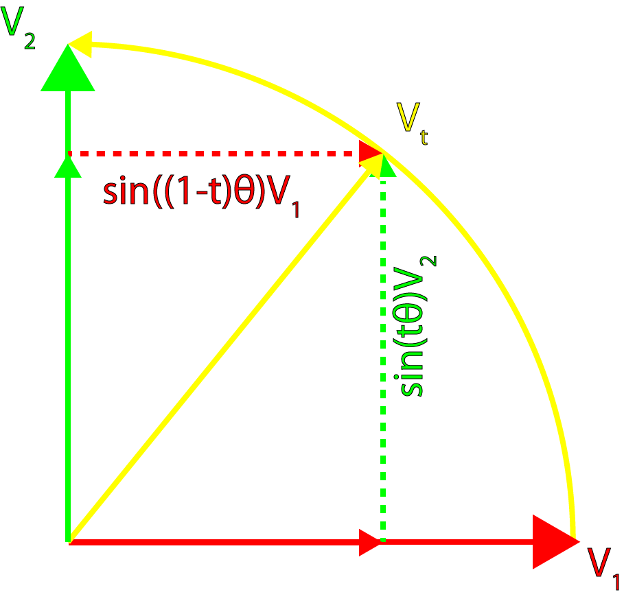
Quaternion Interpolation

This formula can be applied to quaternions without changes:

$$ $$q_t = \ frac {\ sin (1-t) \ theta} {\ sin \ theta} q_1 + \ frac {\ sin {t \ theta}} {\ sin \ theta} q_2$$

And we can get a corner $$$\ theta$ by calculating the dot product $$$q_1$ and $$$q_2$ .

$$ $$\ begin {array} {rcl} \ cos \ theta & = & \ cfrac {q_1 {\ cdot} q_2} {| q_1 || q_2 |} \\ & = & \ cfrac {s_ {1} s_ {2} + x_ {1} x_ {2} + y_ {1} y_ {2} + z_ {1} z_ {2}} {| q_1 || q_2 |} \\ \ theta & = & \ cos ^ {- 1} \ left (\ cfrac {s_ {1} s_ {2} + x_ {1} x_ {2} + y_ {1} y_ {2} + z_ {1} z_ {2}} {| q_1 || q_2 |} \ right) \ end {array}$$

Factors to Consider

This implementation has two problems to consider when using.

First, if the scalar product of quaternions turns out to be a negative value, then the interpolation will go along the “long way” on the four-dimensional sphere, and this is not always desirable. To solve this problem, we can check the result of the scalar product, and if it is negative, then we can take the opposite of one of the orientations. Inverting the scalar and vector parts of the quaternion does not change the orientation it represents, but by doing this, we guarantee that the turn will take place along the “shortest” path.

Another problem arises if the angular difference between $$$q_1$ and $$$q_2$ very small $$$\ sin \ theta$ becomes 0. If this happens, then when dividing by $$$\ sin \ theta$ we can get an uncertain result. In this case, you can return to using linear interpolation between $$$q_1$ and $$$q_2$.

SQUAD

Just as SLERP can be used for interpolation between two quaternions, SQUAD ( S pherical and Quad rangle - spherical and quadrilateral) can be used for smooth interpolation along the turn path.

If we have a number of quaternions:

$$ $$q_1, q_2, q_3, \ cdots, q_ {n-2}, q_ {n-1}, q_ {n}$$

And we defined the "auxiliary" quaternion ( $$$s_i$), which we can consider as an intermediate control point:

$$ $$s_i = \ exp \ left (- \ frac {\ log \ left (q_ {i + 1} q_i ^ {- 1} \ right) + \ log \ left (q_ {i-1} q_i ^ {- 1} \ right)} {4} \ right) q_i$$

Orientation along part of a curve is defined as:

$$ $$q_ {i-1}, q_i, q_ {i + 1}, q_ {i + 2}$$

at time t it gives us:

$$ $$\ mathrm {squad} (q_i, q_ {i + 1}, s_i, s_ {i + 1}, t) = \ mathrm {slerp} (\ mathrm {slerp} (q_i, q_ {i + 1}, t ), \ mathrm {slerp} (s_i, s_ {i + 1}, t), 2t (1-t))$$

Conclusion

Despite the difficulty to understand, when working with turns, quaternions provide several obvious advantages over Euler matrices and angles.

• Interpolation of quaternions using SLERP and SQUAD provides a way to smoothly interpolate between orientations in space.
• Concatenation of turns using quaternions is faster than combining turns expressed in a matrix form.
• For single quaternions-norms, the reciprocal of the rotation is taken by subtracting the vector part of the quaternion. The calculation of the reciprocal of the rotation matrix is ​​much slower if the matrix is ​​not orthonormal (if it is orthonormal, then this is just the matrix transposition).
• The conversion of quaternions to matrices is slightly faster than for Euler angles.
• To describe the rotation, quaternions require only 4 numbers (3, if they are normalized. The real part can be calculated during the execution of the program), while matrices need at least 9 values.

However, along with all the advantages of using quaternions, there are also a few drawbacks.

• Quaternions may become invalid due to a round-off error of floating point numbers; however, this "crept error" can be eliminated by renormalization of quaternion.
• Probably the most significant obstacle to the use of quaternions is the high complexity of their understanding. I hope you solve this problem by reading my article.

There are many mathematical libraries that implement quaternions, and only some of them implement quaternions correctly. In my own experience, a good mathematical library with a qualitative implementation of quaternions is the GLM (OpenGL Math Library). If you want to use quaternions in your own applications, I recommend this library.

Download demo

I created a small demo that demonstrates the use of quaternion to rotate an object in space. The demo was created in Unity 3.5.2, you can download free download this engine and view the source code of the demo. The zip file also contains the Windows binary executable, but in Unity you can build the application for Mac as well.

Understanding Quaternions.zip

Reference materials

Vince, J (2011). Quaternions for Computer Graphics. 1st. ed. London: Springer.

Dunn, F. and Parberry, I. (2002). 3D Math Primer for Graphics and Game Development. 1st. ed. Plano, Texas: Wordware Publishing, Inc.