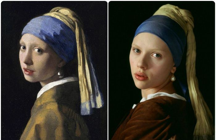
The development of deep neural networks for image recognition inhales new life into already known areas of research in machine learning. One such area is domain adaptation. The essence of this adaptation is to train the model on the data from the source domain (source domain) so that it shows a comparable quality on the target domain (target domain). For example, the source domain can be synthetic data that can be “cheaply” generated, and the target domain is user photos. Then the task of domain adaptation is to train a model on synthetic data that will work well with “real” objects.

In the Vision@Mail.Ru machine vision group, we are working on various applied tasks, and among them there are often those for whom there is little training data. In these cases, the generation of synthetic data and the adaptation of the model trained on them can help greatly. A good applied example of such an approach is the problem of detecting and recognizing products on the shelves in a store. Obtaining photos of such shelves and their markings are quite labor-intensive, but they can be simply generated. Therefore, we decided to dive deeper into the topic of domain adaptation.

Studies in domain adaptation address issues of using the previous experience accumulated by the neural network in a new task. Will the network be able to isolate some features from the source domain and use them in the target domain? Although the neural network in machine learning is only remotely related to neural networks in the human brain, the Holy Grail of artificial intelligence researchers is teaching the neural networks the capabilities that a person has. And people are able to use previous experience and accumulated knowledge to understand new concepts.

In addition, domain adaptation can help solve one of the fundamental problems of deep learning: to train large networks with high recognition quality, a very large amount of data is needed, which in practice is not always available. One solution may be to use domain adaptation methods on synthetic data that can be generated in virtually unlimited quantities.

Quite often in applied tasks there is a case when data are available only from one domain for learning, and the model must be applied on another domain. For example, a network that determines the aesthetic quality of a photograph can be trained on a database available on the web, collected from the site of amateur photographers. And it is planned to use this network on ordinary photos, the quality level of which is on average different from the level of a photo from a specialized photo site. As a solution, you can consider adapting the model to ordinary unpartitioned photos.

Such theoretical and applied issues lie in the domain adaptation domain. In this article, I will talk about the main current research in this area, based on deep learning, and datasets for comparing different methods. The main idea of ​​deep domain adaptation is to train a deep neural network on the source domain, which will translate the image into such a vector representation (embedding) (usually the last layer of the network), which when used on the target domain will result in high quality.

Basic benchmarks

As in any field of machine learning, in a domain adaptation a certain amount of research accumulates over time, which must be compared with each other. For this, the community produces datasets, in the training part of which the models are trained, and in the test part they are compared. Despite the fact that the area of ​​deep domain adaptation research is still relatively young, there are already quite a large number of articles and databases that are used in these articles. I will list the main ones, focusing on the adaptation of the domain of synthetic data to "real".

Numbers

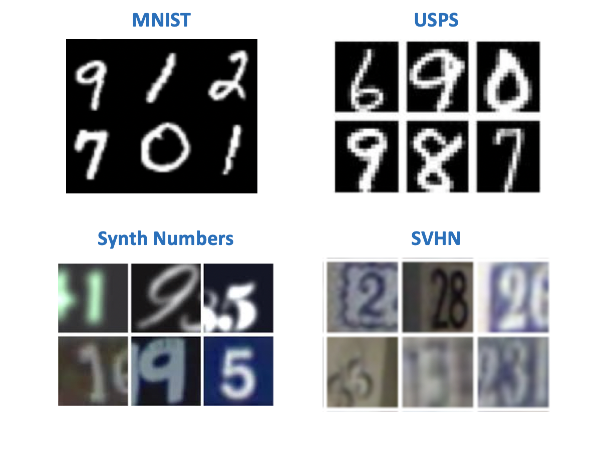
Apparently, according to the tradition instituted by Yann LeKun (one of the pioneers of deep learning, director of Facebook AI Research), in the computer vision the simplest datasets are associated with handwritten numbers or letters. There are several data sets with numbers that originally appeared for experiments with models for image recognition. In the articles on domain adaptation, one can find their most diverse combinations in pairs of source - target domain. Among these:

• MNIST - handwritten numbers, does not need additional submission;
• USPS - handwritten numbers in low resolution;
• SVHN - house numbers with Google Street View;
• Synth Numbers are synthetic numbers, as the name suggests.

From the point of view of the task of learning on synthetic data for use in the "real" world, the pairs of the greatest interest are:

• Source: MNIST, Target: SVHN;
• Source: USPS, Target: MNIST;
• Source: Synth Numbers, Target: SVHN.

Most methods have benchmarks on "digital" datasets. But other types of domains can be found not in all articles.

Office

This dataset contains 31 categories of various items, each of which is presented in 3 domains: an image from Amazon, a photo from a webcam and a photo from a digital camera.

It is useful for checking how the model will react to the addition of the background and the quality of the shooting to the target domain.

Road signs

Another pair of datasets for training a model on synthetic data and applying it on “real” data:

• Source: Synth Signs - images of road signs, generated so that they look like real signs on the street;
• Target: GTSRB is a fairly well-known recognition base containing signs from German roads.

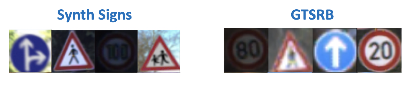
The peculiarity of this pair of databases is that the data from Synth Signs are made quite similar to the “real” data, so the domains are quite close.

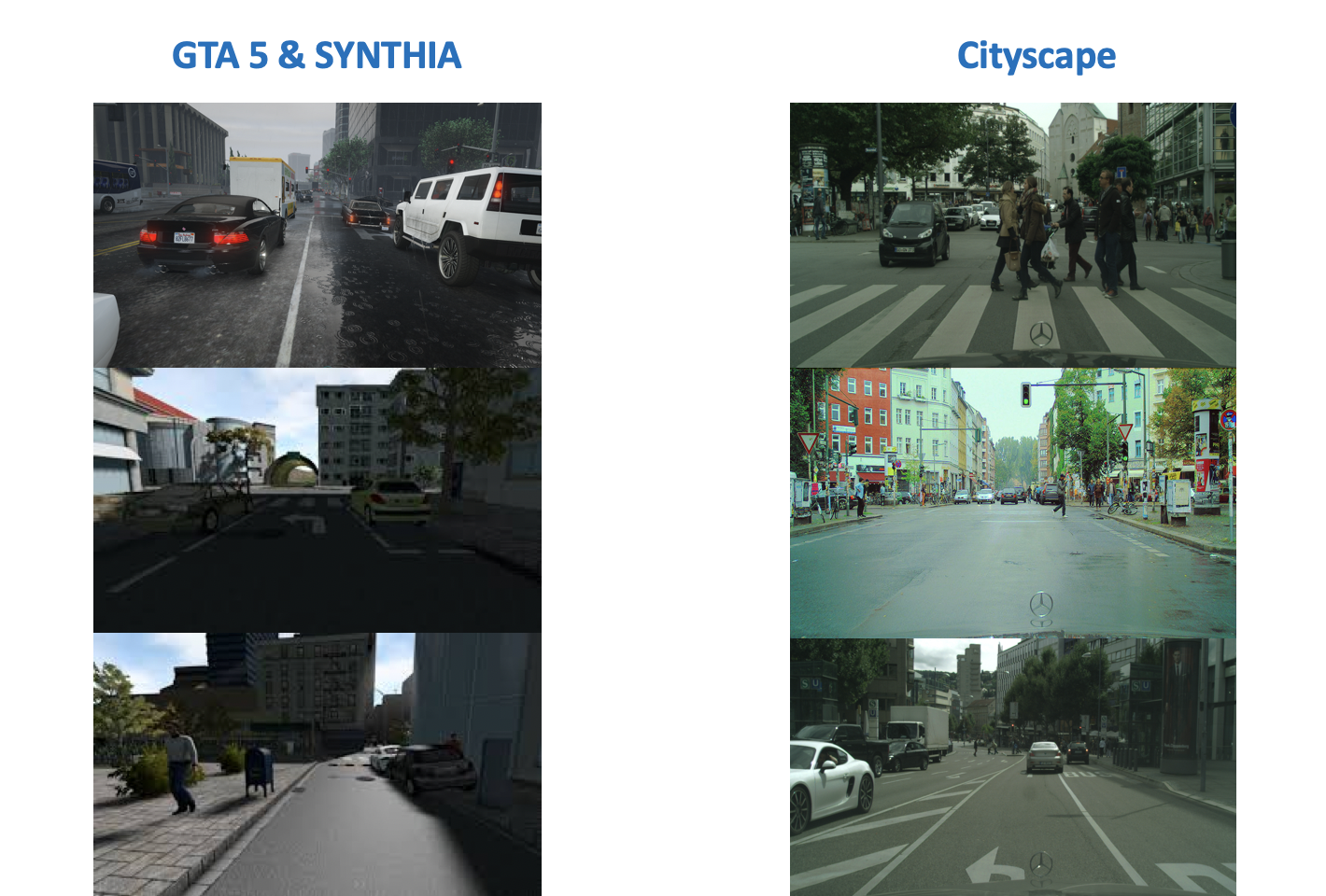
From the car window

Datasets for segmentation. Quite an interesting pair, the most close to real conditions. Baseline data is obtained using the game engine (GTA 5), and target data from real life. Similar approaches are used to train models that are used in autonomous cars.

• SYNTHIA or GTA 5 engine - pictures with city view from the car window, generated using the game engine;
• Cityscapes - photos of the car, made in 50 different cities.

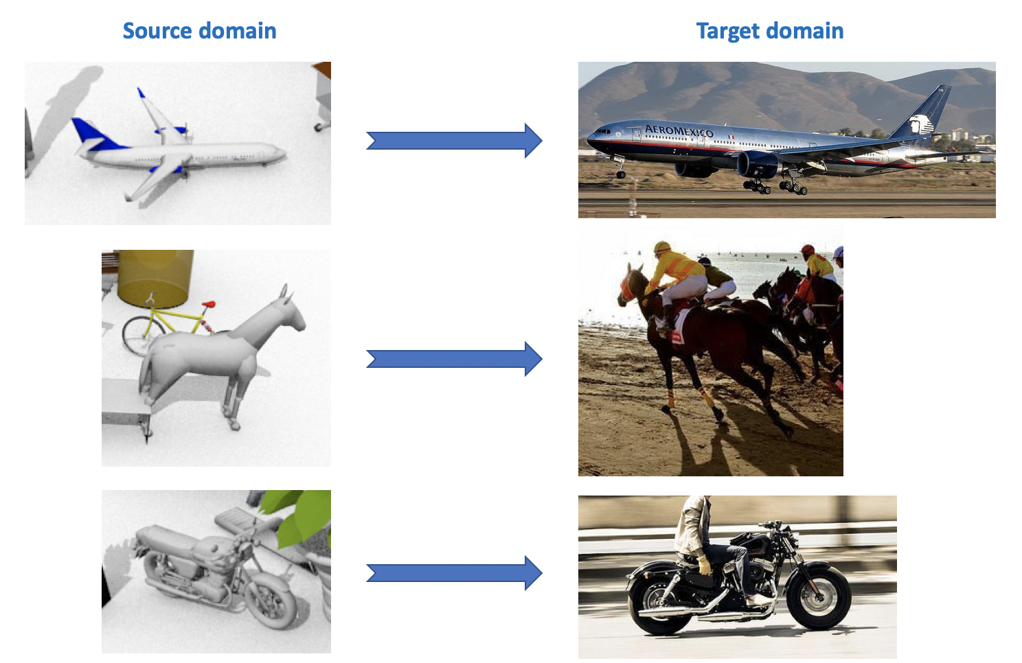
VisDA

This dataset is used in the Visual Domain Adaptation Challenge , which is held as part of the ECCV and ICCV workshop. The source domain contains 12 categories of labeled objects generated using CAD, such as an airplane, a horse, a person, etc. The target domain contains unallocated images from the same 12 categories taken from ImageNet. In the competition, which was held in 2018, the 13th category was added: Unknown.

As can be seen from all of the above, there are quite a lot of interesting and varied datasets for domain adaptation, they can be trained and tested for various tasks (classification, segmentation, detection) and various conditions (synthetic data, photos, street types).

Deep Domain Adaptation

There is a rather extensive and diverse classification of domain adaptation methods (for example , you can get acquainted here ). I will give in this article a simplified division of methods according to their key features. Modern deep domain adaptation methods can be divided into 3 large groups:

• Discrepancy-based : approaches based on minimizing the distance between vector representations on the source and target domains by introducing this distance into the loss function.
• Adversarial-Based : these approaches use a competitive (adversarial) loss function, which appeared in GANs, to train a network that is invariant with respect to the domain. The methods of this family have been actively developed in the last couple of years.
• Mixed methods that do not use adversarial loss, but apply ideas from the discrepancy-based family, as well as the latest developments from deep learning: self-ensembling, new layers, loss functions, etc. These approaches show the best results in the VisDA competition.

From each section we will review several major, in my opinion, results obtained in the last 1-3 years.

Discrepancy-based

When the problem arises of adapting the model to new data, the first thing that comes to mind is the use of fine-tuning, i.e. Additional model training on new data. To do this, you must take into account the measure of discrepancy between domains. This type of domain adaptation can be divided into three approaches: Class Criterion, Statistical criterion and Architecture Criterion.

Class criterion

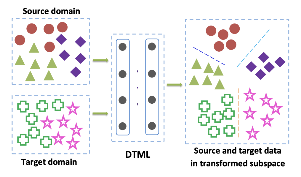
Methods from this family are mainly used when tagged data from the target domain is available to us. One of the popular variants of Class Criterion is the Deep transfer metric learning approach. As the name implies, it is based on metric learning, the essence of which is to teach such a vector representation, derived from a neural network, that representatives of one class will be close to each other in this representation according to a given metric (most often they use $$$L ^ 2$or cosine metrics). The article Deep transfer metric learning (DTML) for the implementation of this approach uses a loss consisting of the sum of the following components:

• The proximity of representatives of one class to each other (intraclass compactness);
• Increasing the distance between representatives of different classes (interclass separability);
• Metric Maximum Mean Discrepancy (MMD) between domains. This metric belongs to the statistical criterion family (see below), but is also used in class criterion.

MMD between domains is written as

$$

$$MMD ^ 2 (D_s, D_t) = \ Vert \ frac {1} {M} \ sum_ {i = 1} ^ M \ phi (x_i ^ s) - \ frac {1} {N} \ sum_ {j = 1} ^ N \ phi (x_j ^ t) \ Vert ^ 2_H,$$

Where $$$\ phi (x)$- this is some core, in our case - vector representation of the network, $$$x_i ^ s, i \ in 1 \ ldots M$- data from the source domain, $$$x_i ^ t, i \ in 1 \ ldots N$- data from the target domain. Thus, while minimizing the MMD metric during training, such a network is selected $$$\ phi (x)$so that its mean vector representations on both domains are close. DTML main idea:

If the data in the target domain is not unmarked (unsupervised domain adaptation), the method described in Mind the Class Weight Bias: Weighted Maximum Mean Discrepancy for the Unsupervised Domain Adaptation suggests teaching the model on the source domain and using it to get pseudo-labels (pseudo- labels) on the target domain. Those. the data from the target domain is run through the network and the result is called pseudo-labels. Then they are used as markup for the target domain, which allows the MMD criterion to be applied to the loss function (with different weights for the components responsible for different domains).

Statistical criterion

Methods related to this family are used to solve the problem of unsupervised domain adaptation. The case when the target domain is unallocated occurs in many problems, and all domain adaptation methods that will be discussed later in this article solve exactly this problem.

Approaches based on statistical criteria attempt to measure the difference between the distribution of the vector representation of the network obtained from the data of the source and target domains. They then use the calculated difference to approximate the two distributions.

One of these criteria is the Maximum Mean Discrepancy (MMD) already described above. Its variants are used in several methods:

• Deep adaptation network (DAN) ;
• Joint adaptation network (JAN) ;
• Residual transfer network (RTN) . RTN shows good results for a pair of MNIST -> SVHN: 90.66% accuracy on the target domain.

Schemes of these three methods are presented below. In them, MMD variants are used to determine the difference between the distributions on the layers of the convolutional neural network applied to the source and target domains. Please note that each of them uses a MMD modification as a loss between layers of convolutional networks (yellow figures in the diagram).

The CORAL (CORrelation ALignment) criterion and its extension with the help of deep Deep CORAL networks are aimed at learning such a representation of the data so that the second-order statistics between the domains coincide as much as possible. For this, the covariance matrices of vector representations of the network are used. The convergence of second-order statistics on both domains in some cases allows for better adaptation results than for MMD.

$$

$$L_ {CORAL} = \ frac {1} {4d ^ 2} \ Vert C_S - C_T \ Vert ^ 2_F,$$

Where $$$|| * || _F ^ 2$- the square of the matrix norm of Frobenius, and $$$C_S$and $$$C_T$- covariance data matrices from the source and target domains, respectively, $$$d$- dimension of the vector representation.

On Office data, average adaptation quality using Deep CORAL for Amazon and Webcam domain pairs: 72.1%. On the Synth Signs -> GTSRB road sign domains, the result is also quite average: 86.9% accuracy on the target domain.

A development of the ideas of MMD and CORAL is the Central Moment Discrepancy (CMD) criterion , which compares the central moments of data from the source and target domains of all orders to $$$K$inclusive ( $$$K$- parameter of the algorithm). At Office, the average CMD adaptation quality for Amazon and Webcam domain pairs is 77.0%.

Architecture criterion

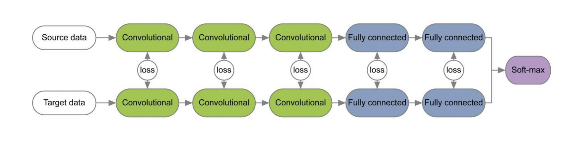
Algorithms of this type are built on the assumption that the basic information that is responsible for adaptation to the new domain is embedded in the parameters of the neural network.

In a number of papers [1] , [2], when learning networks for the source and target domains using loss functions for each pair of layers, information invariant with respect to the domain is studied on the weights of these layers. An example of such architectures is given below.

In the Revisiting Batch Normalization For Practical Domain Adaptation article , the idea was expressed that the weights of the network contain information related to the classes on which the network studies, and the domain information is embedded in the statistics (mean and standard deviation) of Batch Normalization (BN) layers. Therefore, for adaptation, it is necessary to recalculate these statistics on data from the target domain. Using this technique in conjunction with CORAL can improve the quality of adaptation in the Office dataset for couples of the Amazon and Webcam domains to 75.0%. Then it was shown that using the Instance Normalization (IN) layer instead of BN further improves the quality of adaptation. In contrast to BN, which normalizes the input tensor by batch, IN calculates statistics for normalization by channels and, therefore, does not depend on the batch.

Adversarial-Based Approaches

In the last 1-2 years, most of the results in deep domain adaptation are related to the adversarial-based approach. This is largely due to the rapid development and growing popularity of Generative Adversarial Networks (GAN) , because the adversarial-based approach to domain adaptation uses the same competitive (adversarial) objective function when training as GAN. By optimizing it, such deep domain adaptation methods minimize the distance between the empirical distributions of vector data representations on the source and target domains. By training the network in this way, they try to make it invariant with respect to the domain.

GAN consists of two models: generator $$$G$, at the output of which data is obtained from a certain target distribution; and discriminator $$$D$which determines whether the data from the training sample has been input to it or generated using $$$G$. These two models are trained using adversarial objective function:

$$

$$\ min_G \ max_D V (D, G) = \ mathbb {E} _ {x \ sim p_ {data} (x)} [\ log D (x)] + \ mathbb {E} _ {z \ sim p (z)} [1 - \ log D (G (z))].$$

With such training, the generator learns to "deceive" the discriminator, which allows to bring together the distribution of the target and source domains.

There are two big approaches in adversarial-based domain adaptation, which differ in whether or not a generator is used. $$$G$.

Non-Generative Models

A key feature of the methods from this family is the training of a neural network with a vector representation invariant with respect to the source and target domains. Then the network trained in the marked source domain can be used on the target domain, ideally with practically no loss of classification quality.

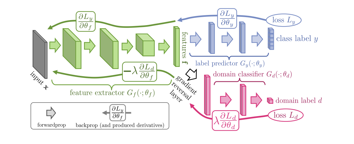
Introduced in 2015, the Domain-Adversarial Training of Neural Networks (DANN) algorithm ( code ) consists of 3 parts:

• The main network, with the help of which a vector representation (feature extractor) is obtained (the green part in the illustration below);
• "Heads" responsible for classification on the source domain (the blue part in the illustration);
• "Heads" that learns to distinguish data from the source domain from the target (the red part in the illustration).

When learning using gradient descent (SGD) (arrows to the input in the illustration), classification and domain loss are minimized. In addition, when the error propagates backward for the “head” responsible for the domains, the Gradient reversal layer (the black part in the illustration) is used, which multiplies the gradient passing through it by a negative constant, increasing the domain loss. This ensures that the distribution of vector representations on both domains become close.

DANN results on benchmarks:

• On a pair of digital domains Synth Numbers -> SVHN: 91.09%.
• On Synth Signs -> GTSRB road signs, it surpasses CORAL with a score of 88.7%.
• On Office data, average adaptation quality for Amazon and Webcam domain pairs: 73.0%.

The next important representative of the non-generative models family is the Adversarial Discriminative Domain Adaptation (ADDA) method ( code ), which implies network separation for the source domain and the network for the target domain. The algorithm consists of the following steps:

1. First, we classify the classifying network on the source domain. We denote its vector representation $$$M_s$, but $$$\ mathbf {X} _s$- source domain.
2. Now we initialize the neural network for the target domain using the trained network from the previous step. Denote it $$$M_t$, but $$$\ mathbf {X} _t$- target domain.
3. Let's move on to the adversarial training: we will train the discriminator $$$D$with fixed $$$M_s$and $$$M_t$using the following objective function:
   
   

   $$

   $$\ min_D L_ {adv_D} (\ mathbf {X} _s, \ mathbf {X} _t, M_s, M_t) = - \ mathbb {E} _ {x_s \ sim \ mathbf {X} _s} [\ log D ( M_s (x_s))] - \ mathbb {E} _ {x_t \ sim \ mathbf {X} _t} [\ log (1 - D (M_t (x_t)))]$$
   
   
4. Freeze discriminator and pre-train $$$M_t$on target domain:
   

   $$

   $$\ min_ {M_s, M_t} L_ {adv_M} (\ mathbf {X} _s, \ mathbf {X} _t, D) = - \ mathbb {E} _ {x_t \ sim \ mathbf {X} _t} [\ log D (M_t (x_t))]$$
   
   

Steps 3 and 4 are repeated several times. The essence of ADDA is that we first train a good classifier on the marked source domain, and then adapt it using adversarial training so that the vector representations of the classifier on both domains are close. Graphically, the algorithm can be represented as follows:

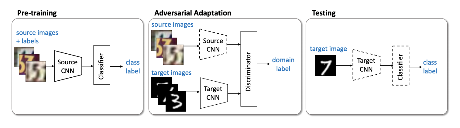
On a pair of digital domains, USPS -> MNIST ADDA showed a result of 90.1% accuracy on the target domain.

The ADDA modification was presented this year at the ICML-2018 conference M-ADDA: Unsupervised Domain Adaptation with Deep Metric Learning ( code ).

Since the main idea of ​​the original algorithm is to bring the vector representations closer to different domains, the authors of M-ADDA use metric learning in order to better divide classes by $$$L ^ 2$-metrics. To do this, at step 1, ADDA, when training the network on the source domain, uses Triplet loss (it simultaneously minimizes the distance between positive examples (from one class) and maximizes between negative ones). As a result of such training, vector representations of data seek to break into $$$K$clusters (where $$$K$- number of classes). For each cluster, its center is calculated. $$$C_j, j \ in 1 \ ldots K$.

Then there is learning as in ADDA, i.e. Steps 2-4 are performed. Only after step 4 is a regularization added, which forces vector representations on the target domain to reach the nearest cluster $$$C_j$, thus providing the best separability of classes in the target domain:

$$

$$\ mathbb {E} _ {x_t \ sim \ mathbf {X} _t} [\ min_j || M_t (x_t) - C_j || ^ 2].$$

The model learning scheme on the target domain is presented below.

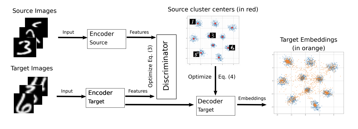
M-ADDA improved the result of the original algorithm on a pair of USPS -> MNIST to 94.0%.

A rather atypical representative of a non-generative family is the Maximum Classifier Discrepancy for Unsupervised Domain Adaptation ( code ) method . He also teaches such vector representations (generator) to be as close as possible to each other on the source and target domains. However, as a discriminator, this method uses the differences in prediction between the two classifiers trained on the generator.

Let the generator $$$G$- this is a kind of convolution network, $$$F_1$and $$$F_2$- two classifiers that use the generator output as an input feature vector. The idea of ​​the method is that $$$G$, $$$F_1$and $$$F_2$are trained on the source domain; then classifiers are trained so as to maximize their disagreement on the target domain; after that the generator is rebuilt so that the disagreement is minimized; and at the end updated $$$F_1$and $$$F_2$.

As can be seen from the description, the algorithm is based on a minimax adversarial-procedure, which should result in a network $$$G$, invariant with respect to the domain.

As a measure of disagreement (Discrepancy Loss) is used

$$

$$d (p_1, p_2) = \ frac {1} {K} \ sum_ {k = 1} ^ K | p_ {1_k} - p_ {2_k} |,$$

Where $$$K$- the number of classes $$$p_ {1_k}$$$$p_ {2_k}$- softmax values $$$k$class for classifiers $$$F_1$and $$$F_2$respectively.

More formally, the method consists of 3 steps:

• A. On the initial domain are trained $$$G$, $$$F_1$and $$$F_2$.
• B. The generator is fixed, and the disagreement of classifiers is maximized on data from the target domain.
• C. Now classifiers are fixed, and generator parameters are trained to minimize Discrepancy Loss.

All three steps are repeated. $$$n$times (algorithm parameter). Steps B and C:

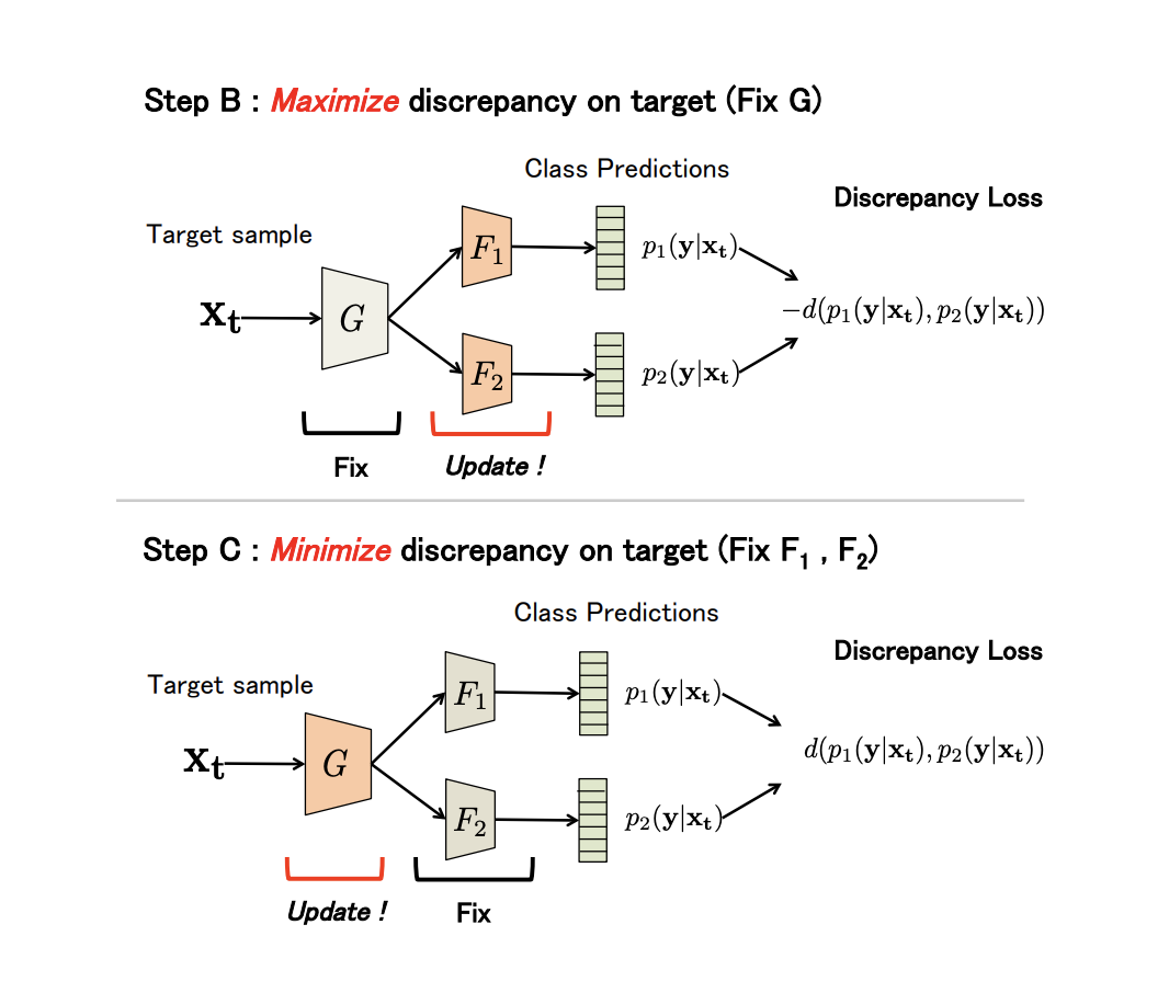
The results of the experiments:

• On a pair of digital domains USPS -> MNIST: 94.1%.
• On the Synth Signs -> GTSRB road signs, the method surpasses all previous ones: 94.4%.
• Based on VisDA, the average value of quality in 12 categories without the Unknown class: 71.9%.
• On a pair of GTA 5 -> Cityscapes: Mean IoU = 39.7%, on Synthia -> Cityscapes: Mean IoU = 37.3%

You can also pay attention to the following interesting algorithms from the family of non-generative models:

• Domain Separation Networks
• A DIRT-T Approach to Unsupervised Domain Adaptation

At this point, let's interrupt.

We considered the basic datasets for domain adaptation, discrepancy-based approaches: class criteria, statistical criteria and architecture criterion, as well as the first family of adversarial-based methods - non-generative. Models from these approaches show themselves well on benchmarks and are applicable for many adaptation tasks. In the next part, we will look at the most complex and effective approaches: generative models and mixed non-adversarial-based methods.