Neural network using TensorFlow: image classification
Hi, Habr! I present to you the translation of the article "Train your first neural network: basic classification" .

This is a neural network training guide for classifying images of clothes, such as sneakers and shirts. To create a neural network, we use python and the TensorFlow library.
Install TensorFlow
To work we need the following libraries:
- numpy (on the command line we write: pip install numpy)
- matplotlib (in the command line we write: pip install matplotlib)
- keras (on the command line we write: pip install keras)
- jupyter (in the command line we write: pip install jupyter)
Using pip: on the command line, write pip install tensorflow
If you get an error, you can download the .whl file and install with pip: pip install path_to_file \ filename_whl
Official TensorFlow Installation Guide
Launch Jupyter. To start the command line write jupyter notebook.
Beginning of work
# import tensorflow as tf from tensorflow import keras import numpy as np import matplotlib.pyplot as plt This tutorial uses the MNIST Fashion dataset, which contains 70,000 grayscale images in 10 categories. Images show individual low-resolution garments (28 by 28 pixels):

We will use 60,000 images for network training and 10,000 images to assess how accurately the network has learned to classify images. You can access Fashion MNIST directly from TensorFlow simply by importing and downloading data:
fashion_mnist = keras.datasets.fashion_mnist (train_images, train_labels), (test_images, test_labels) = fashion_mnist.load_data() Loading the dataset returns four NumPy arrays:
- The train_images and train_labels arrays are the data that the model uses for training
- The test_images and test_labels arrays are used to test the model.
The images are NumPy arrays of 28x28, the pixel values of which are in the range from 0 to 255. Labels (labels) are an array of integers from 0 to 9. They correspond to the class of clothing:
| Tag | Class |
| 0 | T-shirt (T-shirt) |
| one | Trouser (Trousers) |
| 2 | Pullover |
| 3 | Dress |
| four | Coat (Coat) |
| five | Sandal |
| 6 | Shirt (shirt) |
| 7 | Sneaker (Sneakers) |
| eight | Bag |
| 9 | Ankle boot (Ankle boots) |
Class names are not included in the data set, so we write ourselves:
class_names = ['T-shirt/top', 'Trouser', 'Pullover', 'Dress', 'Coat', 'Sandal', 'Shirt', 'Sneaker', 'Bag', 'Ankle boot'] Research data
Consider the format of the data set before training the model.
train_images.shape # 60 000 , 28 x 28 test_images.shape # 10 000 , 28 x 28 len(train_labels) # 60 000 len(test_labels) # 10 000 train_labels # 0 9 ( 3 3 ) Preliminary data processing
Before preparing the model data must be pre-processed. If you check the first image in the training set, you will see that the pixel values are in the range from 0 to 255:
plt.figure() plt.imshow(train_images[0]) plt.colorbar() plt.grid(False) 
We scale these values to a range from 0 to 1:
train_images = train_images / 255.0 test_images = test_images / 255.0 Display the first 25 images from the training set and show the name of the class under each image. Make sure the data is in the correct format.
plt.figure(figsize=(10,10)) for i in range(25): plt.subplot(5,5,i+1) plt.xticks([]) plt.yticks([]) plt.grid(False) plt.imshow(train_images[i], cmap=plt.cm.binary) plt.xlabel(class_names[train_labels[i]]) 
Model building
Neural network construction requires adjustment of model layers.
The main building block of the neural network is the layer. Much of the deep learning consists of combining simple layers. Most layers, such as tf.keras.layers.Dense, have parameters that are studied during training.
model = keras.Sequential([ keras.layers.Flatten(input_shape=(28, 28)), keras.layers.Dense(128, activation=tf.nn.relu), keras.layers.Dense(10, activation=tf.nn.softmax) ]) The first layer in the tf.keras.layers.Flatten network converts the image format from a 2d array (28 by 28 pixels) into a 1d array of 28 * 28 = 784 pixels. This layer has no parameters to learn, it only reformats the data.
The next two layers are tf.keras.layers.Dense. These are tightly connected or fully connected neural layers. The first layer of Dense contains 128 nodes (or neurons). The second (and last) level is a layer with 10 nodes tf.nn.softmax, which returns an array of ten probability estimates, the sum of which is 1. Each node contains a rating that indicates the probability that the current image belongs to one of 10 classes.
Compiling the model
Before the model is ready to learn, it will need a few more settings. They are added during the model compilation phase:
- Loss function (loss function) - measures how accurate a model is during training
- The optimizer is how the model is updated based on the data it sees and the loss function.
- Metrics (metrics) - used to monitor the stages of training and testing
model.compile(optimizer=tf.train.AdamOptimizer(), loss='sparse_categorical_crossentropy', metrics=['accuracy']) Model training
Learning the neural network model requires the following steps:
- Submission of model learning data (in this example, the train_images and train_labels arrays)
- Model learns to associate images and tags
- We ask the model to make predictions about the test set (in this example, the test_images array). We check the consistency of the predictions of the tags from the tags array (in this example, the test_labels array)
To start learning, call the model.fit method:
model.fit(train_images, train_labels, epochs=5) 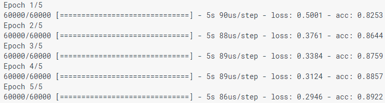
When modeling a model, indicators of losses (loss) and accuracy (acc) are displayed. This model achieves an accuracy of about 0.88 (or 88%) according to training data.
Accuracy Assessment
Compare how the model works in the test dataset:
test_loss, test_acc = model.evaluate(test_images, test_labels) print('Test accuracy:', test_acc) 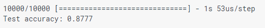
It turns out that the accuracy in the test dataset is slightly less accurate in the training set. This gap between training accuracy and testing accuracy is an example of retraining. Retraining is when a machine learning model works worse with new data than with learning data.
Forecasting
We use the model to predict some images.
predictions = model.predict(test_images) Here the model predicted the label for each image in the test set. Let's look at the first prediction:
predictions[0] 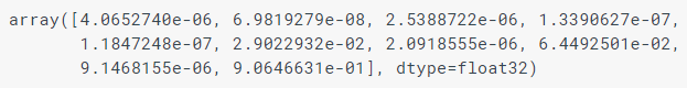
Prediction is an array of 10 numbers. They describe the “confidence” of the model that the image matches each of the 10 different items of clothing. We can see which label has the highest confidence value:
np.argmax(predictions[0]) #9 Thus, the model is most confident that this image is the Ankle boot (Boots), or class_names [9]. And we can check the test tag to make sure that it’s correct:
test_labels[0] #9 We write functions to visualize these predictions.
def plot_image(i, predictions_array, true_label, img): predictions_array, true_label, img = predictions_array[i], true_label[i], img[i] plt.grid(False) plt.xticks([]) plt.yticks([]) plt.imshow(img, cmap=plt.cm.binary) predicted_label = np.argmax(predictions_array) if predicted_label == true_label: color = 'blue' else: color = 'red' plt.xlabel("{} {:2.0f}% ({})".format(class_names[predicted_label], 100*np.max(predictions_array), class_names[true_label]), color=color) def plot_value_array(i, predictions_array, true_label): predictions_array, true_label = predictions_array[i], true_label[i] plt.grid(False) plt.xticks([]) plt.yticks([]) thisplot = plt.bar(range(10), predictions_array, color="#777777") plt.ylim([0, 1]) predicted_label = np.argmax(predictions_array) thisplot[predicted_label].set_color('red') thisplot[true_label].set_color('blue') Let's look at the 0th image, predictions, and an array of predictions.
i = 0 plt.figure(figsize=(6,3)) plt.subplot(1,2,1) plot_image(i, predictions, test_labels, test_images) plt.subplot(1,2,2) plot_value_array(i, predictions, test_labels) 
Construct several images with their predictions. The correct prediction marks are blue, and the incorrect prediction marks are red. Note that this may be wrong, even when he is very confident.
num_rows = 5 num_cols = 3 num_images = num_rows*num_cols plt.figure(figsize=(2*2*num_cols, 2*num_rows)) for i in range(num_images): plt.subplot(num_rows, 2*num_cols, 2*i+1) plot_image(i, predictions, test_labels, test_images) plt.subplot(num_rows, 2*num_cols, 2*i+2) plot_value_array(i, predictions, test_labels) 
Finally, we use the trained model to make a prediction about a single image.
# img = test_images[0] The tf.keras models are optimized to make forecasts for batch or collection. Therefore, although we use one image, we need to add it to the list:
# , img = (np.expand_dims (img, 0)) Image Forecast:
predictions_single = model.predict(img) print(predictions_single) 
plot_value_array(0, predictions_single, test_labels) _ = plt.xticks(range(10), class_names, rotation=45) 
np.argmax(predictions_single[0]) As before, the model predicts label 9.
If you have questions, write in the comments or in private messages.
')
Source: https://habr.com/ru/post/426797/
All Articles