Neurotic Bikes: Genesis
The other day, Youtube thought it would seem interesting to me a video called “AI Learns to play Hill Climb Racing”. It's funny, because a couple of minutes before that, I committed another change to the project, where my colleagues and I, in the breaks between work and work, solve exactly this problem. No “AI” in that video , however, was revealed - the author entertained the public with pampering with Box2D and calmed down on that. Nevertheless, I propose to consider this fact as convincing evidence of the relevance of the topic and disassemble the structure of our rattles.
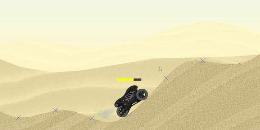
Briefly about the task: the vehicle - in our case it is either Alien, or the Zinger sewing machine on wheels, let's call it simply “agent” - must travel along the perichind noise of the same name from the dunes from start to finish. This is what an agent looks like in his sandbox:
')
An agent who has touched the back of the track or does not demonstrate proper zeal in moving towards the goal is removed from the track.
We will solve the problem using neural networks, but optimized by a genetic algorithm (GA) - this process is called neuroevolution . We used the NEAT method (NeuroEvolution of Augmenting Topologies), invented by Kenneth Stanley and Risto Miikkulainen at the beginning of the century [1] : firstly, he had a good account of important problems for the national economy, secondly, to start working on the project in our country already had its own framework implementing NEAT. So, to be honest, we didn’t choose the solution method - rather, we chose a task where we could drive the ready one.
The figure shows an approximate scheme of the work of genetic algorithms:
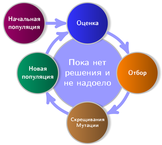
It is seen that any decent GA starts with the initial population (the population is a set of potential solutions). Let us create it and at the same time get acquainted with the first principle of NEAT . According to this principle, all agents of the starting population should have the simplest, “minimal” topology of the neural network. What does it have to do with topology? The fact is that in NEAT, along with the optimization of link weights, the network architecture evolves. This, by the way, eliminates the need to design it for a task. To go from simple architectures to complex ones is not only logical, but also practical (less search space), and therefore it is necessary to begin with the minimum possible topology - this is how the authors of the method argued.
For our and all similar cases, this minimal topology is derived from the following considerations. To do something meaningful agent need:
The first role is played by the sensors - the neurons of the input layer, to which we will provide useful information to the agent. The neurons of the output layer will process the data from the sensors. For interaction with the environment, actuators are responsible - devices that perform mechanical actions in response to a signal from "their" neuron of the output layer. The general principle of building the initial configuration is thus the following: we determine the sensors and actuators, initiate one neuron for the actuator, all sensors and another special neuron - displacement neuron ( bias , about it - below) are connected with random weights with all neurons output layer. Something like this:
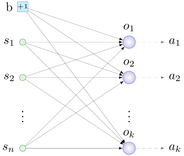
b - bias, s - sensors, o - neurons of the output layer, a - actuators, n - number of sensors, k - number of actuators
And this is what the minimum NA looks like for our task:
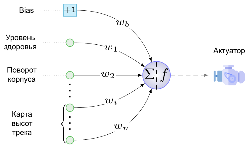
We have only one actuator - this is the engine of our wheeled creation. Shoot, jump and play the tune it still does not know how. On the engine from a single neuron of the output layer (it is embarrassing to call it a layer), this value is given here:


Here w b is the value of the weight of the connection going from bias to the output neuron, multiplied by what every bias “produces”, i.e. +1, s i is the value normalized to the range [0,1] on the i-th sensor, w i is the weight value of the connection from the i-th sensor to the output neuron, and f is the activation function.
As an activation function, we use this fantasy on the subject of softsign:


- it demonstrated the best performance in the tests of a neuroevolutionist well-known in narrow circles [2] . And to compare the soft-looking softness of the curves and the symmetry of the graph of this function with the angular-crooked Leaky ReLU makes no sense at all:

This figure shows the agent's reaction to different values of the activation function. At close to unity values, the engine turns the wheels clockwise, accelerating the agent forward and strongly deflecting the body backwards, so that the mentally minded, but the brave quickly overturned on his back and die. At values close to 0, the opposite is true, and at a value of 0.5, the agent motor does not work.
The same figure shows the role of the displacement neuron - the weight of the connection going from it to the neuron of the output layer is responsible, as follows from (1), for the magnitude and direction of displacement f (x) along the abscissa axis. The dotted line in the figure shows the graph of the activation function when w b = -1. It turns out that even in the absence of a signal on the sensors, an agent with such a connection would rather quickly go back: f (x) = f (-1 + 0) ≈0.083 <0.5. In general, the horizontal shift of the function values allows the bias communication to be fine (well, or thick — depending on weight) to adjust the response of the engine to all sensor values and the weights of their connections at once. It seems that a new dimension has been added to the search space (the “correct” value for w b will have to be searched for), but the benefit in the form of an additional degree of freedom from the possibility of such displacements outweighs.
Great, we introduced the neural networks of agents of a future initial population. But NEAT is a genetic algorithm, and it works with genotypes — the structures that make up networks or, more generally, phenotypes in the decoding process. Since we started with the phenotype, let's do everything backwards: we will try to encode the network presented above in the genotype. Here, one cannot do without the second principle of NEAT , the main essence of which is as follows: in the genotype, in addition to the structure of the neural network and the weights of its connections, information is stored about the history of the origin of all its elements. With the exception of this historical aspect, the phenotype is encoded in the genotype almost “one to one”, therefore, we will illustrate the second principle for the time being with fragments of neural networks.
The value of this principle is difficult to overestimate - it provides agents with the possibility of sexual reproduction. The topic is rather delicate, therefore we will first consider asexual reproduction. It happens like this: a copy of all the genes of the agent is made, one of several types of changes is made on them - mutations . The following mutations are possible in our version of NEAT:
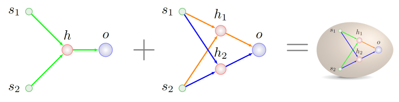
The first three types of mutations are simple and understandable without further explanation. The neuron insertion is shown in the figure below, it always takes place in place of the existing connection, the connection is removed, and two new ones appear in its place:
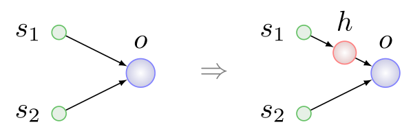
Here h is a hidden ( hidden ) neuron.
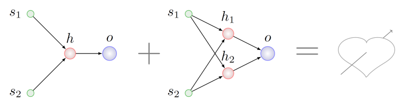
Two agents participate in sexual reproduction or interbreeding - parents, and as a result a third one appears - a child. In the process of the formation of a child's genotype, an exchange occurs, let's say, with the same within the meaning of the genes or groups of genes of the parents. The second principle is just needed to search for genes with the same meaning.
Imagine that we want to cross agents with genotypes that have undergone different mutation series from the list above:
It seems logical to look for some common from the point of view of topology fragments from both parents and take a piece of these fragments for the genotype of the unborn child. It will be difficult to do this, even NP is difficult in the general case, but suppose we managed. In this case, we find that in the parent on the right there are two subgraphs isomorphic to the graph of the left parent. In the figure below, the arcs of these subgraphs are highlighted in different colors:
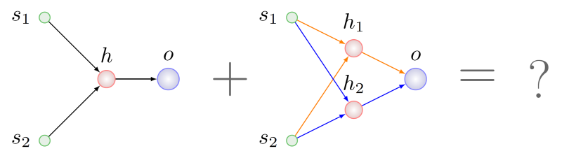
Which one to choose for recombination with the genes of the left parent?
Let us turn to the history of the emergence of these genotypes:
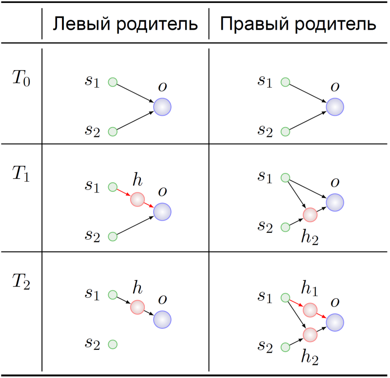
Both ancestors of the parent agents started, as expected, with a minimum NA (T 0 ). Their genomes somehow mutated there, and at the time T 1 in the ancestor of the left parent, a hidden neuron was inserted into the connection s 1 -> o. At this dramatic moment, the genes encoding the connections s 1 -> h and h -> o acquire their meaning in the ancestor of the left parent: the substitution of the connection s 1 -> o .
The s 1 -> h 1 and h 1 -> o genes in the genotype of the right parent at the time point T 2 had the same meaning. The further destinies of our ancestors do not particularly interest us - we already know what we can mix with:
The next time it will be possible to make out how to write a genetic history, all the more so since we have some small finds in this area, they are connected with the adaptation of the original technique to a stable reproduction scheme.
It's time to wrap up. The article began with Youtube - they will complete it. In the early version of the simulator, a colleague who wrote the track generation code ended it with a bottomless abyss. The reaction of the neural network, which has evolved for a long time in the presence of the earth, under the wheels, can be called a “pattern break” for such a design of its small universe:
An extensive collection of other anecdotal stories from the life of cybernaturalists can be found in [3] .
[one] KO Stanley and R .. Miikkulainen, "Evolving Neural Networks through Augmenting Topologies" Evolutionary Computation, vol. 10, no. 2, pp. 99-127, 2002.
[2] C. Green, “A Review of Activation Functions in SharpNEAT,” 19 June 2017.
[3] J. Lehman et al, “The Surprising Creativity of the Digital Evolution: A Collection of Anecdotes from the Evolutionary Computation and Artificial Life Research Communities,” arXiv: Neural and Evolutionary Computing, 2018.
Briefly about the task: the vehicle - in our case it is either Alien, or the Zinger sewing machine on wheels, let's call it simply “agent” - must travel along the perichind noise of the same name from the dunes from start to finish. This is what an agent looks like in his sandbox:
')
An agent who has touched the back of the track or does not demonstrate proper zeal in moving towards the goal is removed from the track.
We will solve the problem using neural networks, but optimized by a genetic algorithm (GA) - this process is called neuroevolution . We used the NEAT method (NeuroEvolution of Augmenting Topologies), invented by Kenneth Stanley and Risto Miikkulainen at the beginning of the century [1] : firstly, he had a good account of important problems for the national economy, secondly, to start working on the project in our country already had its own framework implementing NEAT. So, to be honest, we didn’t choose the solution method - rather, we chose a task where we could drive the ready one.
The figure shows an approximate scheme of the work of genetic algorithms:
It is seen that any decent GA starts with the initial population (the population is a set of potential solutions). Let us create it and at the same time get acquainted with the first principle of NEAT . According to this principle, all agents of the starting population should have the simplest, “minimal” topology of the neural network. What does it have to do with topology? The fact is that in NEAT, along with the optimization of link weights, the network architecture evolves. This, by the way, eliminates the need to design it for a task. To go from simple architectures to complex ones is not only logical, but also practical (less search space), and therefore it is necessary to begin with the minimum possible topology - this is how the authors of the method argued.
For our and all similar cases, this minimal topology is derived from the following considerations. To do something meaningful agent need:
- have environmental and state data,
- process this information
- interact with your world.
The first role is played by the sensors - the neurons of the input layer, to which we will provide useful information to the agent. The neurons of the output layer will process the data from the sensors. For interaction with the environment, actuators are responsible - devices that perform mechanical actions in response to a signal from "their" neuron of the output layer. The general principle of building the initial configuration is thus the following: we determine the sensors and actuators, initiate one neuron for the actuator, all sensors and another special neuron - displacement neuron ( bias , about it - below) are connected with random weights with all neurons output layer. Something like this:
b - bias, s - sensors, o - neurons of the output layer, a - actuators, n - number of sensors, k - number of actuators
And this is what the minimum NA looks like for our task:
We have only one actuator - this is the engine of our wheeled creation. Shoot, jump and play the tune it still does not know how. On the engine from a single neuron of the output layer (it is embarrassing to call it a layer), this value is given here:
Here w b is the value of the weight of the connection going from bias to the output neuron, multiplied by what every bias “produces”, i.e. +1, s i is the value normalized to the range [0,1] on the i-th sensor, w i is the weight value of the connection from the i-th sensor to the output neuron, and f is the activation function.
As an activation function, we use this fantasy on the subject of softsign:
- it demonstrated the best performance in the tests of a neuroevolutionist well-known in narrow circles [2] . And to compare the soft-looking softness of the curves and the symmetry of the graph of this function with the angular-crooked Leaky ReLU makes no sense at all:
This figure shows the agent's reaction to different values of the activation function. At close to unity values, the engine turns the wheels clockwise, accelerating the agent forward and strongly deflecting the body backwards, so that the mentally minded, but the brave quickly overturned on his back and die. At values close to 0, the opposite is true, and at a value of 0.5, the agent motor does not work.
The same figure shows the role of the displacement neuron - the weight of the connection going from it to the neuron of the output layer is responsible, as follows from (1), for the magnitude and direction of displacement f (x) along the abscissa axis. The dotted line in the figure shows the graph of the activation function when w b = -1. It turns out that even in the absence of a signal on the sensors, an agent with such a connection would rather quickly go back: f (x) = f (-1 + 0) ≈0.083 <0.5. In general, the horizontal shift of the function values allows the bias communication to be fine (well, or thick — depending on weight) to adjust the response of the engine to all sensor values and the weights of their connections at once. It seems that a new dimension has been added to the search space (the “correct” value for w b will have to be searched for), but the benefit in the form of an additional degree of freedom from the possibility of such displacements outweighs.
Great, we introduced the neural networks of agents of a future initial population. But NEAT is a genetic algorithm, and it works with genotypes — the structures that make up networks or, more generally, phenotypes in the decoding process. Since we started with the phenotype, let's do everything backwards: we will try to encode the network presented above in the genotype. Here, one cannot do without the second principle of NEAT , the main essence of which is as follows: in the genotype, in addition to the structure of the neural network and the weights of its connections, information is stored about the history of the origin of all its elements. With the exception of this historical aspect, the phenotype is encoded in the genotype almost “one to one”, therefore, we will illustrate the second principle for the time being with fragments of neural networks.
The value of this principle is difficult to overestimate - it provides agents with the possibility of sexual reproduction. The topic is rather delicate, therefore we will first consider asexual reproduction. It happens like this: a copy of all the genes of the agent is made, one of several types of changes is made on them - mutations . The following mutations are possible in our version of NEAT:
- change in bond weight,
- removing a connection
- adding a connection
- neuron insertion.
The first three types of mutations are simple and understandable without further explanation. The neuron insertion is shown in the figure below, it always takes place in place of the existing connection, the connection is removed, and two new ones appear in its place:
Here h is a hidden ( hidden ) neuron.
Two agents participate in sexual reproduction or interbreeding - parents, and as a result a third one appears - a child. In the process of the formation of a child's genotype, an exchange occurs, let's say, with the same within the meaning of the genes or groups of genes of the parents. The second principle is just needed to search for genes with the same meaning.
Imagine that we want to cross agents with genotypes that have undergone different mutation series from the list above:
It seems logical to look for some common from the point of view of topology fragments from both parents and take a piece of these fragments for the genotype of the unborn child. It will be difficult to do this, even NP is difficult in the general case, but suppose we managed. In this case, we find that in the parent on the right there are two subgraphs isomorphic to the graph of the left parent. In the figure below, the arcs of these subgraphs are highlighted in different colors:
Which one to choose for recombination with the genes of the left parent?
Let us turn to the history of the emergence of these genotypes:
Both ancestors of the parent agents started, as expected, with a minimum NA (T 0 ). Their genomes somehow mutated there, and at the time T 1 in the ancestor of the left parent, a hidden neuron was inserted into the connection s 1 -> o. At this dramatic moment, the genes encoding the connections s 1 -> h and h -> o acquire their meaning in the ancestor of the left parent: the substitution of the connection s 1 -> o .
The s 1 -> h 1 and h 1 -> o genes in the genotype of the right parent at the time point T 2 had the same meaning. The further destinies of our ancestors do not particularly interest us - we already know what we can mix with:
The next time it will be possible to make out how to write a genetic history, all the more so since we have some small finds in this area, they are connected with the adaptation of the original technique to a stable reproduction scheme.
It's time to wrap up. The article began with Youtube - they will complete it. In the early version of the simulator, a colleague who wrote the track generation code ended it with a bottomless abyss. The reaction of the neural network, which has evolved for a long time in the presence of the earth, under the wheels, can be called a “pattern break” for such a design of its small universe:
An extensive collection of other anecdotal stories from the life of cybernaturalists can be found in [3] .
Sources
Source: https://habr.com/ru/post/426783/
All Articles