Graphics in Julia. Strange patterns, the reflection of a triangle from a straight line and the construction of the normals of a spherical cat in a vacuum

We continue to get acquainted with a very young, but incredibly beautiful and powerful programming language Julia . The six-year beta is finally over, so now you can not be afraid of changes in syntax. And while everyone is arguing, it’s good or bad to start indexing from one, the excited community has been actively messed up: new libraries are coming out, old ones are being updated, serious projects are being launched, and students are actively taught this language at universities. So let's not fall behind! Brew tea stronger, because this night we will code!
Preparation for work
There is a small overview in Russian, as well as on Habré there is an acquaintance with the language and installation guide . Again, I draw attention to the need for the Windows Management Framework , there will be problems with loading packages.
The JuliaPRO package after the update now includes only Juno . But personally, I prefer Jupyter : there were no problems with it on a laptop, plus it’s convenient to work in the browser and immediately create notes and formulas, in general, ideal for creating reports, slides or manuals.
- Download the latest version of Julia from the official site
- The link to the jupiter in the set of Anaconda is given above, I used the one that was in the old JuliaPRO
- Launch Julia. It is already possible to fully use the language, but only in interpreter mode. Execute commands:
julia>] pkg> add IJulia pkg> build IJulia # build - Now creation of Julia 1.0.1 file is available in Jupyter.
There are several packages for Julia, the most successful ones are included in Plots as backends. Plots.jl is a meta-language for plotting a graph: that is, an interface for various graph libraries. Thus, Plots.jl actually just interprets your commands, and then creates graphs using any kind of graph library. These background graphic libraries are called backends. The best part is that you can use many different graphic libraries with the syntax Plots.jl , and we will also see that Plots.jl adds new functions to each of these libraries!
To install packages, run the commands in REPL, Juno, or Jupyter:
# Pkg.add("Plots") # 0.7.0 julia>] pkg>add Plots pkg>add GR pkg>add PyPlot pkg>add Gadfly pkg>add PlotlyJS pkg>add UnicodePlots It is not necessary to install all the packages, but you should know that each of them has its own characteristics . I prefer plotlyjs () : although it does not differ in speed, but very interactive. There is a zoom, movement along the plane, as well as the ability to save a file, and if you save the Jupyter document as html, all possibilities will be preserved. So you can add to the site or make an interactive presentation. More information on the pages: Plots , Gadfly
Endless pattern based on prime numbers
Implemented the idea of an article on Habré . In a few words: what if we take the coordinate of a point and between an abscissa and ordinate, apply some operation, say, XOR or bitwise AND , and then check the number for simplicity or for belonging to Fibonacci numbers, and if the answer is positive, fill the point with one color, and with a negative in the other? Check:
using Plots plotlyjs() function eratosphen(n, lst) # ar = [i for i=1:n] ar[1] = 0 for i = 1:n if ar[i] != 0 push!(lst, ar[i]) for j = i:i:n ar[j] = 0 end end end end ertsfn = [] eratosphen(1000, ertsfn) # print(ertsfn) # print( size(ertsfn) ) # -> 168 N = 80 M = 80 W1 = [in( x % y, ertsfn) for x = 1:N, y = 1:M]; W2 = [x % y for x = 1:N, y = 1:M]; p1 = spy(W1, title = "x % y is prime?") p2 = spy(W2, title = "x % y") plot(p1, p2, layout=(2),legend=false) 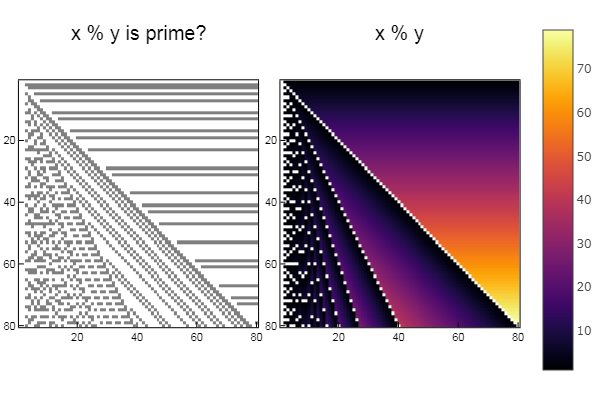
W1 = [in( x + y, ertsfn) for x = 1:N, y = 1:M]; W2 = [x + y for x = 1:N, y = 1:M]; p1 = spy(W1, title = "x + y is prime?") p2 = spy(W2, title = "x + y") plot(p1, p2, layout=(2),legend=false) 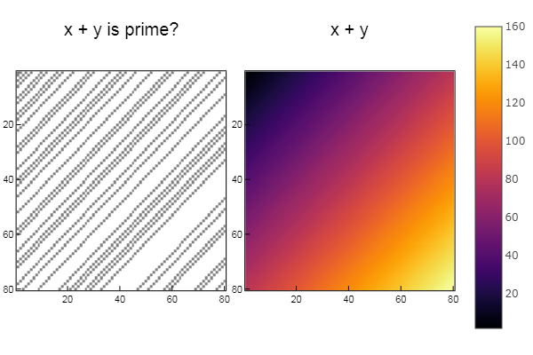
W1 = [in( x | y, ertsfn) for x = 1:N, y = 1:M]; W2 = [x | y for x = 1:N, y = 1:M]; p1 = spy(W1, title = "x | y is prime?") p2 = spy(W2, title = "x | y") plot(p1, p2, layout=(2),legend=false) 
W1 = [in( x & y, ertsfn) for x = 1:N, y = 1:M]; W2 = [x & y for x = 1:N, y = 1:M]; p1 = spy(W1, title = "x & y is prime?") p2 = spy(W2, title = "x & y") plot(p1, p2, layout=(2),legend=false) 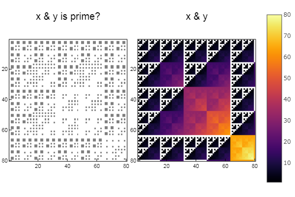
W1 = [in( xor(x, y), ertsfn) for x = 1:N, y = 1:M]; W2 = [xor(x, y) for x = 1:N, y = 1:M]; p1 = spy(W1, title = "x xor y is prime?") p2 = spy(W2, title = "x xor y") plot(p1, p2, layout=(2),legend=false) 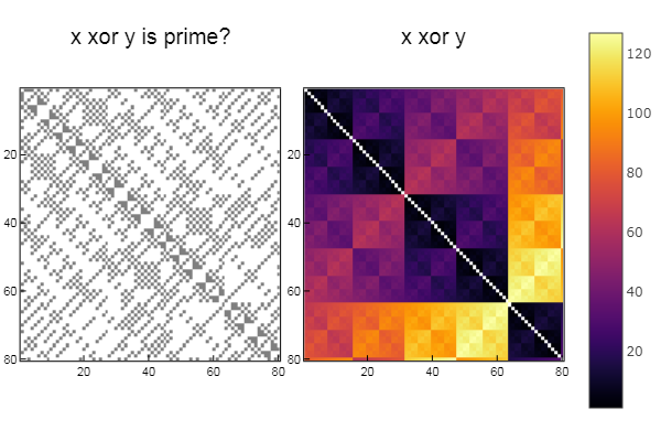
It is possible, as usual, to form a series with something like:
function fib(n) a = 0 b = 1 for i = 1:n a, b = b, a + b end return a end fbncc = fib.( [i for i=1:10] ) But let's use the matrix representation ( more ):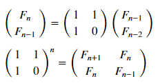
matr_fib = n -> [1 1; 1 0]^(n-1) # , n-1 mfbnc = [ matr_fib( i )[1,1] for i=1:17]; # 1,1 n- N = 100 M = N W1 = [in( x % y, mfbnc) for x = 1:N, y = 1:M]; W2 = [in( x | y, mfbnc) for x = 1:N, y = 1:M]; p1 = spy(W1, title = "x % y ∈ fibonacci?") p2 = spy(W2, title = "x | y ∈ fibonacci?") plot(p1, p2, layout=(2),legend=false) 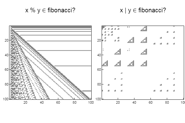
W1 = [in( xor(x, y), mfbnc) for x = 1:N, y = 1:M]; W2 = [in( x & y, mfbnc) for x = 1:N, y = 1:M]; p1 = spy(W1, title = "x xor y ∈ fibonacci?") p2 = spy(W2, title = "x & y ∈ fibonacci?") plot(p1, p2, layout=(2),legend=false) 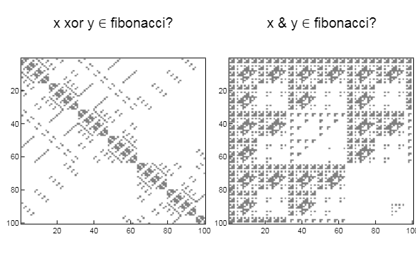
The reflection of the figure is relatively straightforward.
This type of display is determined by the matrix:
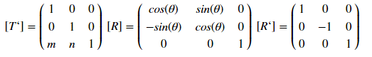
where [T '], [R] and [R'], respectively, of the matrix of displacement, rotation and reflection. How it works? Using an example of an offset, for a point with coordinates (x, y), the offset by m by ix and by n by the game will be determined by the transformation:
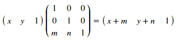
These matrices allow conversions for different polygons, the main thing is to write down the coordinates under each other and not forget about the column of ones at the end. Thus [T]:
- shifts the line at the origin along with the polygon to be transformed
- turns it to coincide with the X axis
- reflects all points of the polygon relative to X
- then reverse and translate
In more detail the topic is disclosed in the book of Rogers D., Adams J. Mathematical foundations of computer graphics
Now code it!
using Plots plotlyjs() f = x -> 0.4x + 2 # # X = [2 4 2 2]' Y = [4 6 6 4]' xs = [-2; 7] # ys = f(xs) inptmtrx = [ XY ones( size(X, 1), 1 ) ] # m = 0 n = -f(0) # Y displacement = [1 0 0; 0 1 0; mn 1] a = (ys[2]-ys[1]) / (xs[2]-xs[1]) # θ = -atan(a) rotation = [cos(θ) sin(θ) 0; -sin(θ) cos(θ) 0; 0 0 1] reflection = [1 0 0; 0 -1 0; 0 0 1] T = displacement * rotation * reflection * rotation^(-1) * displacement^(-1) # outptmtrx = inptmtrx * T plot( X, Y) plot!( xs, ys ) plot!( outptmtrx[:,1], outptmtrx[:,2] ) 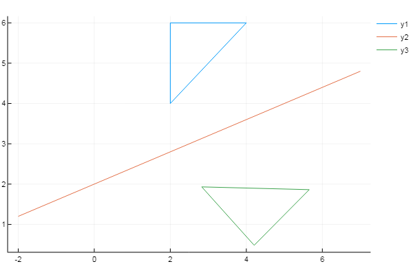
Interesting fact: if you get rid of the Greek characters and replace the first line with
function y=f(x,t) y=0.4*x + 2 endfunction, brackets [] framing indices of arrays on () , and rafts on plot( X, Y, xs, ys, trianglenew(:,1), trianglenew(:,2) ) , then this code runs in Scilab .
Work with three-dimensional graphics
Some of the listed packages support the construction of three-dimensional graphs. But separately I would like to mention Makie’s rather powerful visualization tool , which works in conjunction with the GLFW and GLAbstraction packages that implement the OpenGL features in julia. More information about Makie . His approbation hide under
using Makie N = 51 x = linspace(-2, 2, N) y = x z = (-x .* exp.(-x .^ 2 .- (y') .^ 2)) .* 4 scene = wireframe(x, y, z) xm, ym, zm = minimum(scene.limits[]) scene = surface!(scene, x, y, z) contour!(scene, x, y, z, levels = 15, linewidth = 2, transformation = (:xy, zm)) scene 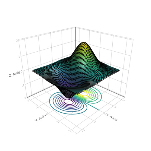
wireframe(Makie.loadasset("cat.obj")) 
using FileIO scene = Scene(resolution = (500, 500)) catmesh = FileIO.load(Makie.assetpath("cat.obj"), GLNormalUVMesh) mesh(catmesh, color = Makie.loadasset("diffusemap.tga")) 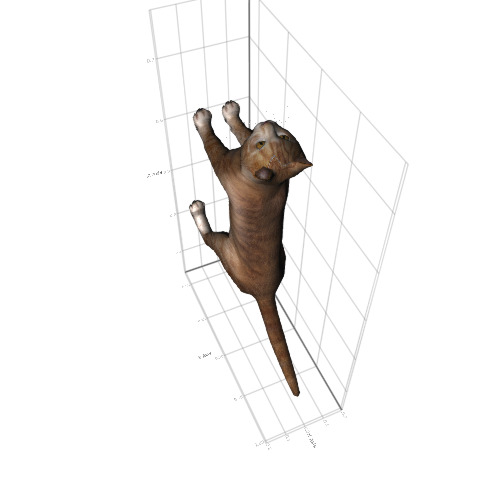
x = Makie.loadasset("cat.obj") mesh(x, color = :black) pos = map(x.vertices, x.normals) do p, n p => p .+ (normalize(n) .* 0.05f0) end linesegments!(pos, color = :blue) 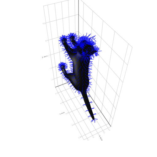
On this with all the graphics. Interactivity, animation, 3d, big data or fast construction of the simplest graphs - constantly evolving packages will satisfy almost every taste and need, moreover, everything is quite easy to master. Feel free to download practical tasks and continues to comprehend Julia!
UPD: All the above listings are made in Jupyter with julia 0.6.4. Unfortunately, some functions of the Plots metapacket were either removed or renamed, so that we continue to follow the updates, but in the meantime, the spy is completely replaced:
julia> using GR julia> Z = [x | y for x = 1:40, y = 1:40]; julia> heatmap(Z) ')
Source: https://habr.com/ru/post/426387/
All Articles