Symbolic solution of linear differential equations and systems by the Laplace transform method using SymPy

The implementation of algorithms in Python using symbolic calculations is very convenient when solving problems of mathematical modeling of objects defined by differential equations. To solve such equations, Laplace transformations are widely used, which, to put it simply, allow us to reduce the problem to solving the simplest algebraic equations.

In this publication, I propose to consider the functions of the direct and inverse Laplace transform from the SymPy library, which allow using the Laplace method to solve differential equations and systems using Python tools.

The Laplace method itself and its advantages in solving linear differential equations and systems are widely covered in the literature, for example, in the popular publication [1]. In the book, the Laplace method is given for implementation in licensed software packages Mathematica, Maple and MATLAB (which implies the acquisition of this software by an educational institution) on selected examples by the author.

Let us try today to consider not a separate example of solving a learning problem using Python, but a general method for solving linear differential equations and systems using the functions of the direct and inverse Laplace transform. At the same time, we keep the learning moment: the left side of a linear differential equation with Cauchy conditions will be formed by the student himself, and the routine part of the problem, consisting in the direct Laplace transform of the right side of the equation, will be performed using the laplace_transform () function.
')

The authorship history of the Laplace transform

Laplace transformations (images by Laplace) have an interesting history. For the first time, the integral in the definition of the Laplace transform appeared in one of the works of L. Euler. However, in mathematics it is customary to call a method or theorem the name of the mathematician who discovered it after Euler. Otherwise, there would be several hundred different Euler theorems.

In this case, the following after Euler was the French mathematician Pierre Simon de Laplace (Pierre Simon de Laplace (1749-1827)). It was he who used such integrals in his work on probability theory. The Laplace itself did not use the so-called “operational methods” for finding solutions to differential equations based on Laplace transforms (Laplace images). These methods were actually discovered and promoted by practical engineers, especially by the English electrical engineer Oliver Heaviside (1850-1925). Long before the validity of these methods was rigorously proved, operational calculus was successfully and widely applied, although its legitimacy was largely questioned even at the beginning of the twentieth century, and very fierce debates were held on this topic.

The functions of the direct and inverse Laplace transform

The direct Laplace transform function:
sympy.integrals.transforms. laplace_transform (t, s, ** hints).
The laplace_transform () function performs the Laplace transformations of the function f (t) of a real variable into the function F (s) of a complex variable, so that:
$F (s) = i n t_{0}^{\infty} f (t) e^{- s t} d t .$
$F (s) = \ int_ {0} ^ {∞} f (t) e ^ {- st} dt.$

This function returns (F, a, cond) , where F (s) is the Laplace transform of the function f (t) , a <Re (s) is the half-plane where F (s) is defined, and cond are the auxiliary conditions for the convergence of the integral.
If the integral cannot be computed in a closed form, this function returns an uncomputed object's LaplaceTransform .
If you set the option noconds = True , the function returns only F (s) .
Inverse Laplace transform function:

sympy.integrals.transforms. inverse_laplace_transform (F, s, t, plane = None, ** hints).

The inverse_laplace_transform () function performs the inverse Laplace transformation of the function of the complex variable F (s) into the function f (t) of a real variable, so that:
$f (t) = f r a c 1 2 p i i i n t_{c - \infty c d o t i}^{c + \infty c d o t i} e^{s t} F (s) d s .$
$f (t) = \ frac {1} {2 \ pi i} \ int_ {c-∞ \ cdot i} ^ {c + ∞ \ cdot i} e ^ {st} F (s) ds.$

If the integral cannot be computed in a closed form, this function returns an uncalculated InverseLaplaceTransform object.

Inverse Laplace transform on the example of determining the transition characteristics of regulators

The transfer function of the PID controller is [2]:

W (s) = (1 + f r a c K_{d} c d o t T_{d} c d o t s 1 + T_{d} c d o t s) c d o t K_{p} c d o t (1 + f r a c 1 T_{i} c d o t s) c d o t f r a c 1 s .

$W (s) = (1+ \ frac {K_ {d} \ cdot T_ {d} \ cdot s} {1 + T_ {d} \ cdot s}) \ cdot K_ {p} \ cdot (1+ \ frac {1} {T_ {i} \ cdot s}) \ cdot \ frac {1} {s}.$

We write a program for obtaining equations for the transient characteristics of the PID and PI controllers for the reduced transfer function, and additionally derive the time taken to perform the inverse visual Laplace transform.

Text of the program

#   : from sympy import * import time import matplotlib.pyplot as plt import numpy as np start = time.time() #   : var('s Kp Ti Kd Td') #      : var('t', positive=True) Kp = 2 Ti = 2 Kd = 4 Td = Rational(1, 2) #   -   s: fp = (1 + (Kd * Td * s) / (1 + Td*s)) * Kp * (1 + 1/(Ti*s)) * (1/s) #   -, #     : ht = inverse_laplace_transform(fp, s, t) Kd = 0 #   - (Kd = 0)   s: fpp = (1 + (Kd * Td * s) / (1 + Td*s)) * Kp * (1 + 1/(Ti*s)) * (1/s) #   -, #     : htt = inverse_laplace_transform(fpp, s, t) stop = time.time() print ('     : %ss' % N((stop-start), 3)) #      : f = lambdify(t, ht, 'numpy') F = lambdify(t, htt, 'numpy') tt = np.arange(0.01, 20, 0.05) #  : plt.title('   \n   : \n  - W(s)=%s \n  - W(s)=%s' % (fp, fpp)) plt.plot(tt, f(tt), color='r', linewidth=2, label='-: h(t)=%s' % ht) plt.plot(tt, F(tt), color='b', linewidth=2, label='-: h(t)=%s' % htt) plt.grid(True) plt.legend(loc='best') plt.show()

We get:

Laplace reverse visual conversion time: 2.68 s

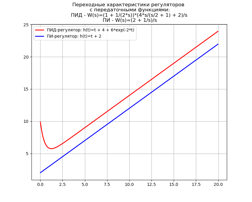
The inverse Laplace transform is often used in the synthesis of ACS, where Python can replace expensive software “monsters” such as MathCAD, so the use of the inverse transform is of practical importance.

Laplace transformation from higher order derivatives for solving the Cauchy problem

In continuation of our discussion there will be an application of Laplace transformations (images according to Laplace) to search for solutions of a linear differential equation with constant coefficients of the form

a c d o t x^{'} (t) + b c d o t x^{'} (t) + c c d o t x (t) = f (t) . (1)

$a \ cdot x '(t) + b \ cdot x' (t) + c \ cdot x (t) = f (t). (1)$

If a and b are constants, then

L \ left \ {a \ cdot f (t) + b \ cdot q (t) \ right \} = a \ cdot L \ left \ {f (t) \ right \} + b \ cdot L \ left \ {q (t) \ right \} (2)

$L \ left \ {a \ cdot f (t) + b \ cdot q (t) \ right \} = a \ cdot L \ left \ {f (t) \ right \} + b \ cdot L \ left \ {q (t) \ right \} (2)$

for all s such that both Laplace transforms (Laplace images) of the functions f (t) and q (t) exist.

Check the linearity of the direct and inverse Laplace transforms using the previously considered functions laplace_transform () and inverse_laplace_transform () . To do this, as an example, take f (t) = sin (3t) , q (t) = cos (7t) , a = 5 , b = 7 and use the following program.

Text of the program

 from sympy import* var('sa b') var('t', positive=True) a = 5 f = sin(3*t) b = 7 q = cos(7*t) #   a*L{f(t)}: L1 = a * laplace_transform(f, t, s, noconds=True) #   b*L{q(t)}: L2 = b*laplace_transform(q, t, s, noconds=True) #  a*L{f(t)}+b*L{q(t)}: L = factor(L1 + L2) print (L) #   L{a*f(t)+b*q(t)}: LS = factor(laplace_transform(a*f + b*q, t, s, noconds=True)) print (LS) print (LS == L) #   a* L^-1{f(t)}: L_1 = a * inverse_laplace_transform(L1/a, s, t) #   b* L^-1{q(t)} L_2 = b * inverse_laplace_transform(L2/b, s, t) # a* L^-1{f(t)}+b* L^-1{q(t)}: L_S = L_1 + L_2 print (L_S) #   L^-1{a*f(t)+b*q(t)}: L_1_2 = inverse_laplace_transform(L1 + L2, s, t) print (L_1_2) print (L_1_2 == L_S)

We get:

(7 * s ** 3 + 15 * s ** 2 + 63 * s + 735) / ((s ** 2 + 9) * (s ** 2 + 49))
(7 * s ** 3 + 15 * s ** 2 + 63 * s + 735) / ((s ** 2 + 9) * (s ** 2 + 49))
True
5 * sin (3 * t) + 7 * cos (7 * t)
5 * sin (3 * t) + 7 * cos (7 * t)

The code also demonstrates the uniqueness of the inverse Laplace transform.

Assuming that

q (t) = f^{'} (t)

$q (t) = f '(t)$ satisfies the conditions of the first theorem, it will follow from this theorem that:

L \ left \ {f '' (t) \ right \} = L \ left \ {q '(t) \ right \} = sL \ left \ {q (t) \ right \} - q (0) = sL \ left \ {f '(t) \ right \} - f' (0) = s \ left [sL \ left \ {f (t) -f (0) \ right \} \ right],

$L \ left \ {f '' (t) \ right \} = L \ left \ {q '(t) \ right \} = sL \ left \ {q (t) \ right \} - q (0) = sL \ left \ {f '(t) \ right \} - f' (0) = s \ left [sL \ left \ {f (t) -f (0) \ right \} \ right],$

and thus,

L \ left \ {f '' (t) \ right \} = s ^ {2} \ cdot F (s) -s \ cdot f (0) -f '(0).

$L \ left \ {f '' (t) \ right \} = s ^ {2} \ cdot F (s) -s \ cdot f (0) -f '(0).$

Repeating this calculation gives

L \ left \ {f '' '(t) \ right \} = sL \ left \ {f' '(t) \ right \} - f' '(0) = s ^ {3} F (s) -s ^ {2} f (0) -sf '(0) -f' '(0).

$L \ left \ {f '' '(t) \ right \} = sL \ left \ {f' '(t) \ right \} - f' '(0) = s ^ {3} F (s) -s ^ {2} f (0) -sf '(0) -f' '(0).$

After a finite number of such steps, we obtain the following generalization of the first theorem:

L \ left \ {f ^ {(n)} (t) \ right \} = s ^ {n} L \ left \ {f (t) \ right \} - s ^ {n-1} f (0 ) -s ^ {n-2} f '(0) - \ cdot \ cdot \ cdot -f ^ {(n-1)} (0) =

$L \ left \ {f ^ {(n)} (t) \ right \} = s ^ {n} L \ left \ {f (t) \ right \} - s ^ {n-1} f (0 ) -s ^ {n-2} f '(0) - \ cdot \ cdot \ cdot -f ^ {(n-1)} (0) =$

= s^{n} F (s) - s^{n - 1} f (0) - c d o t c d o t c d o t - s f^{(n - 2)} (0) - f^{(n - 1)} (0) . (3)

$= s ^ {n} F (s) -s ^ {n-1} f (0) - \ cdot \ cdot \ cdot -sf ^ {(n-2)} (0) -f ^ {(n- 1)} (0). (3)$

Applying relation (3), which contains the Laplace-derived derivatives of the sought-for function with initial conditions, to equation (1), one can obtain its solution using the method specially developed in our department with the active support of Scorobey for the SymPy library.

Method for solving linear differential equations and systems of equations based on Laplace transforms using the SymPy library

To demonstrate the method, we use a simple differential equation that describes the motion of a system consisting of a material point of a given mass, fixed on a spring, to which an external force is applied. The differential equation and the initial conditions for such a system are:

x^{″} + 4 x = s i n (3 t); x (0) = 1.2; x^{'} (0) = 1, (4)

$x '' + 4x = \ sin (3t); x (0) = 1.2; x '(0) = 1, (4)$

Where

x (0)

$x (0)$ - given the initial position of the mass,

x^{'} (0)

$x '(0)$ - reduced initial mass velocity.

A simplified physical model defined by equation (4) with non-zero initial conditions [1]:

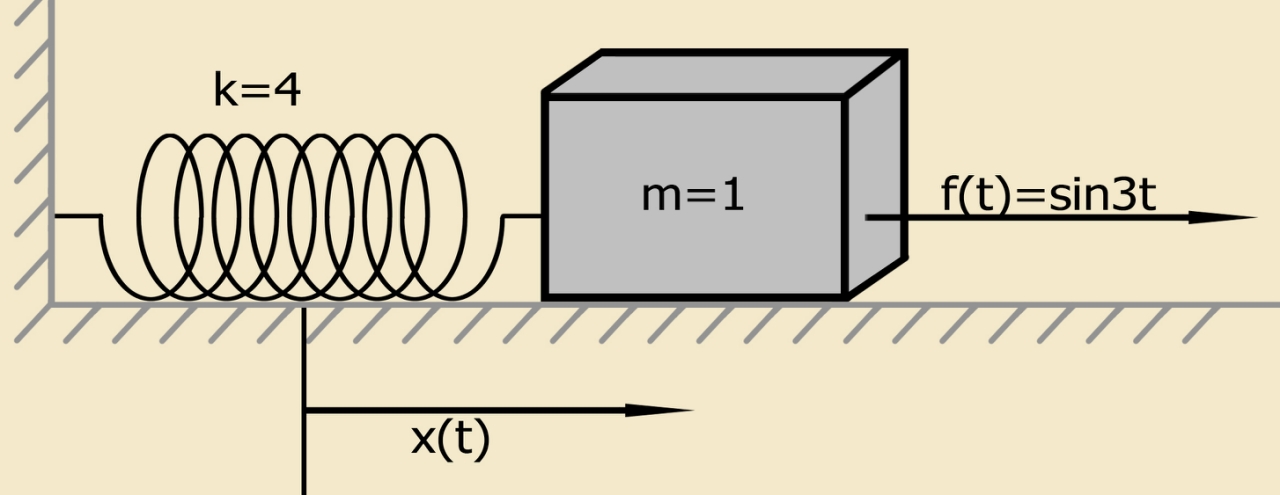
A system consisting of a material point of a given mass fixed on a spring satisfies the Cauchy problem (a problem with initial conditions). The material point of a given mass is initially at rest in the position of its equilibrium.

To solve this and other linear differential equations using the Laplace transform method, it is convenient to use the following system, obtained from relations (3):

L \ left \ {f ^ {IV} (t) \ right \} = s ^ {4} \ cdot F (s) -s ^ {3} \ cdot f (0) -s ^ {2} \ cdot f ^ {I} (0) -s \ cdot f ^ {II} (0) -f ^ {III} (0),

$L \ left \ {f ^ {IV} (t) \ right \} = s ^ {4} \ cdot F (s) -s ^ {3} \ cdot f (0) -s ^ {2} \ cdot f ^ {I} (0) -s \ cdot f ^ {II} (0) -f ^ {III} (0),$

L \ left \ {f ^ {III} (t) \ right \} = s ^ {3} \ cdot F (s) -s ^ {2} \ cdot f (0) -s \ cdot f ^ {I } (0) -f ^ {II} (0),

$L \ left \ {f ^ {III} (t) \ right \} = s ^ {3} \ cdot F (s) -s ^ {2} \ cdot f (0) -s \ cdot f ^ {I } (0) -f ^ {II} (0),$

L \ left \ {f ^ {II} (t) \ right \} = s ^ {2} \ cdot F (s) -s \ cdot f (0) -f ^ {I} (0),

$L \ left \ {f ^ {II} (t) \ right \} = s ^ {2} \ cdot F (s) -s \ cdot f (0) -f ^ {I} (0),$

L \ left \ {f ^ {I} (t) \ right \} = s \ cdot F (s) -f (0), L \ left \ {f (t) \ right \} = F (s) .

$L \ left \ {f ^ {I} (t) \ right \} = s \ cdot F (s) -f (0), L \ left \ {f (t) \ right \} = F (s) .$

L \ left \ {f (t) \ right \} = F (s). (5)

$L \ left \ {f (t) \ right \} = F (s). (5)$

The sequence of the SymPy solution is as follows:

load the required modules and explicitly define character variables:

 from sympy import * import numpy as np import matplotlib.pyplot as plt var('s') var('t', positive=True) var('X', cls=Function)

specify the version of the sympy library to take into account its features. To do this, enter the following lines:
```
 import SymPy print ('  sympy – %' % (sympy._version_)) 
```
According to the physical meaning of the problem, the time variable is determined for the region including zero and positive numbers. We set the initial conditions and the function on the right side of equation (4) with its subsequent Laplace transform. For initial conditions, you must use the Rational function, since the use of decimal rounding leads to an error.
```
 #    : x0 = Rational(6, 5) #   : x01 = Rational(1, 1) g = sin(3*t) Lg = laplace_transform(g, t, s, noconds=True) 
```
using (5), we rewrite the Laplace-transformed derivatives appearing in the left side of equation (4), forming the left side of this equation from them, and compare the result with its right side:
```
 d2 = s**2*X(s) - s*x0 - x01 d0 = X(s) d = d2 + 4*d0 de = Eq(d, Lg) 
```
solve the resulting algebraic equation for the transformation X (s) and perform the inverse Laplace transformation:
```
 rez = solve(de, X(s))[0] soln = inverse_laplace_transform(rez, s, t) 
```
we move from work in the SymPy library to the NumPy library:
```
 f = lambdify(t, soln, 'numpy') 
```

We build the graph in the usual way for Python:

 x = np.linspace(0, 6*np.pi, 100) plt.title(',     \n  :\n  (t)=%s' % soln) plt.grid(True) plt.xlabel('t', fontsize=12) plt.ylabel('x(t)', fontsize=12) plt.plot(x, f(x), 'g', linewidth=2) plt.show()

Full text of the program:

 from sympy import * import numpy as np import matplotlib.pyplot as plt import sympy var('s') var('t', positive=True) var('X', cls=Function) print ("  sympy – %s" % (sympy.__version__)) #       : x0 = Rational(6, 5) #       : x01 = Rational(1, 1) g = sin(3*t) #   : Lg = laplace_transform(g, t, s, noconds=True) d2 = s**2*X(s) - s*x0 - x01 d0 = X(s) d = d2 + 4*d0 de = Eq(d, Lg) #   : rez = solve(de, X(s))[0] #   : soln = inverse_laplace_transform(rez, s, t) f = lambdify(t, soln, "numpy") x = np.linspace(0, 6*np.pi, 100) plt.title(',     \n  :\n  (t)=%s' % soln) plt.grid(True) plt.xlabel('t', fontsize=12) plt.ylabel('x(t)', fontsize=12) plt.plot(x, f(x), 'g', linewidth=2) plt.show()

We get:
Sympy library version - 1.3

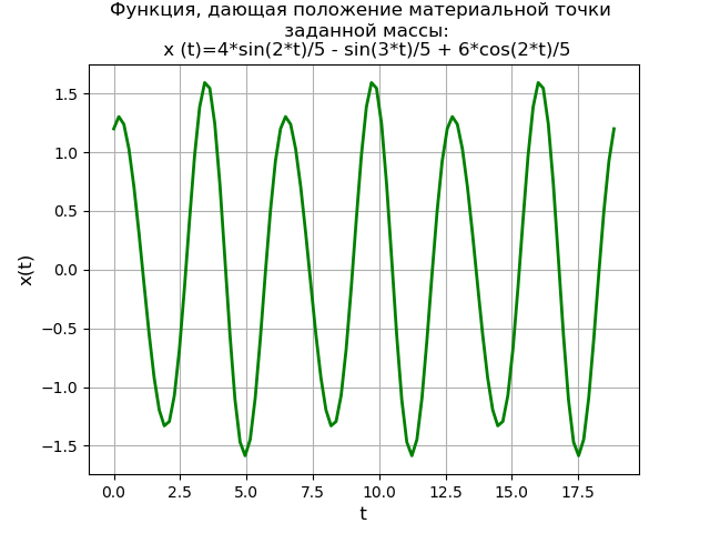
The graph of the periodic function, giving the position of the material point of a given mass. The Laplace transform method using the SymPy library gives a solution not only without the need to first find the general solution of a homogeneous equation and a particular solution to the original inhomogeneous differential equation, but also without the need to use the method of elementary fractions and Laplace tables.

At the same time, the educational value of the solution method is preserved due to the need to use system (5) and transition to NumPy to study the solution using more productive methods.

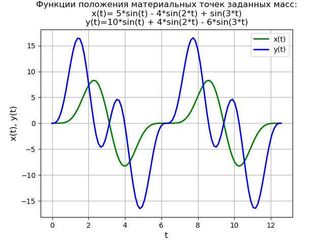
To further demonstrate the method, we solve a system of differential equations:

b e g i n c a s e s 2 x^{″} + 6 x - 2 = 0, y^{'} - 2 x + 2 y = 40 c d o t s i n (3 t), e n d c a s e s (6)

$\ begin {cases} 2x '' + 6x-2 = 0, \\ y '- 2x + 2y = 40 \ cdot \ sin (3t), \ end {cases} (6)$
with initial conditions

x (0) = y (0) = y^{'} (0) = 0.

$x (0) = y (0) = y '(0) = 0.$

A simplified physical model defined by the system of equations (6) with zero initial conditions:

Thus, the force f (t) is suddenly applied to the second material point of a given mass at time t = 0 , when the system is at rest in its equilibrium position.

The solution of the system of equations is identical to the previously considered solution of the differential equation (4), therefore, I quote the program text without explanation.

Text of the program

 from sympy import * import numpy as np import matplotlib.pyplot as plt var('s') var('t ', positive=True) var('X Y', cls=Function) x0 = 0 x01 = 0 y0 = 0 y01 = 0 g = 40 * sin(3*t) Lg = laplace_transform(g, t, s, noconds=True) de1 = Eq(2*(s**2*X(s) - s*x0 - x01) + 6*X(s) - 2*Y(s)) de2 = Eq(s**2*Y(s) - s*y0 - y01 - 2*X(s) + 2*Y(s) - Lg) rez = solve([de1, de2], X(s), Y(s)) rezX = expand(rez[X(s)]) solnX = inverse_laplace_transform(rezX, s, t) rezY = expand(rez[Y(s)]) solnY = inverse_laplace_transform(rezY, s, t) f = lambdify(t, solnX, "numpy") F = lambdify(t, solnY, "numpy") x = np.linspace(0, 4*np.pi, 100) plt.title('     :\nx(t)=%s\ny(t)=%s' % (solnX, solnY)) plt.grid(True) plt.xlabel('t', fontsize=12) plt.ylabel('x(t), y(t)', fontsize=12) plt.plot(x, f(x), 'g', linewidth=2, label='x(t)') plt.plot(x, F(x), 'b', linewidth=2, label='y(t)') plt.legend(loc='best') plt.show()

We get:

For non-zero initial conditions, the program text and function graph will look like this:

Text of the program

 from sympy import * import numpy as np import matplotlib.pyplot as plt var('s') var('t', positive=True) var('X Y', cls=Function) x0 = 0 x01 = -1 y0 = 0 y01 = -1 g = 40 * sin(t) Lg = laplace_transform(g, t, s, noconds=True) de1 = Eq(2*(s**2*X(s) - s*x0 - x01) + 6*X(s) - 2*Y(s)) de2 = Eq(s**2*Y(s) - s*y0 - y01 - 2*X(s) + 2*Y(s) - Lg) rez = solve([de1, de2], X(s), Y(s)) rezX = expand(rez[X(s)]) solnX = (inverse_laplace_transform(rezX, s, t)).evalf().n(3) rezY = expand(rez[Y(s)]) solnY = (inverse_laplace_transform(rezY, s, t)).evalf().n(3) f = lambdify(t, solnX, "numpy") F = lambdify(t, solnY, "numpy") x = np.linspace(0, 4*np.pi, 100) plt.title('     :\nx(t)= %s \ny(t)=%s' % (solnX, solnY)) plt.grid(True) plt.xlabel('t', fontsize=12) plt.ylabel('x(t), y(t)', fontsize=12) plt.plot(x, f(x), 'g', linewidth=2, label='x(t)') plt.plot(x, F(x), 'b', linewidth=2, label='y(t)') plt.legend(loc='best') plt.show()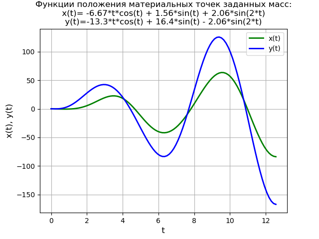

Consider the solution of a fourth-order linear differential equation with zero initial conditions:

x^{(4)} + 2 c d o t x^{″} + x = 4 c d o t t c d o t e^{t};

$x ^ {(4)} + 2 \ cdot x '' + x = 4 \ cdot t \ cdot e ^ {t};$

x (0) = x^{'} (0) = x^{″} (0) = x^{(3)} (0) = 0.

$x (0) = x '(0) = x' '(0) = x ^ {(3)} (0) = 0.$

Program text:

 from sympy import * import numpy as np import matplotlib.pyplot as plt var('s') var('t', positive=True) var('X', cls=Function) #  : x0 = 0 x01 = 0 x02 = 0 x03 = 0 g = 4*t*exp(t) #   : Lg = laplace_transform(g, t, s, noconds=True) d4 = s**4*X(s) - s**3*x0 - s**2*x01 - s*x02 - x03 d2 = s**2*X(s) - s*x0 - x01 d0 = X(s) d = factor(d4 + 2*d2 + d0) de = Eq(d, Lg) #   : rez = solve(de, X(s))[0] #   : soln = inverse_laplace_transform(rez, s, t) f = lambdify(t, soln, "numpy") x = np.linspace(0, 6*np.pi, 100) plt.title(':\n  (t)=%s\n' % soln, fontsize=11) plt.grid(True) plt.xlabel('t', fontsize=12) plt.ylabel('x(t)', fontsize=12) plt.plot(x, f(x), 'g', linewidth=2) plt.show()

Decision graph:

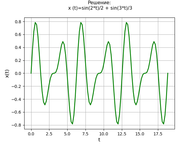
Solve a fourth order linear differential equation:

x^{(4)} + 13 x^{″} + 36 x = 0;

$x ^ {(4)} + 13x '' + 36x = 0;$
with initial conditions

x (0) = x^{″} (0) = 0

$x (0) = x '' (0) = 0$ ,

x^{'} (0) = 2

$x '(0) = 2$ ,

x^{(3)} (0) = - $ 1

$x ^ {(3)} (0) = - $ 1$ .

Program text:

 from sympy import * import numpy as np import matplotlib.pyplot as plt var('s') var('t', positive=True) var('X', cls=Function) #  : x0 = 0 x01 = 2 x02 = 0 x03 = -13 d4 = s**4*X(s) - s**3*x0 - s**2*x01 - s*x02 - x03 d2 = s**2*X(s) - s*x0 - x01 d0 = X(s) d = factor(d4 + 13*d2 + 36*d0) de = Eq(d, 0) #   : rez = solve(de, X(s))[0] #   : soln = inverse_laplace_transform(rez, s, t) f = lambdify(t, soln, "numpy") x = np.linspace(0, 6*np.pi, 100) plt.title(':\n  (t)=%s\n' % soln, fontsize=11) plt.grid(True) plt.xlabel('t', fontsize=12) plt.ylabel('x(t)', fontsize=12) plt.plot(x, f(x), 'g', linewidth=2) plt.show()

Decision graph:

TAC functions

For having an analytical solution of ODE and ODE systems, the dsolve () function is used:
sympy.solvers.ode. dsolve (eq, func = None, hint = 'default', simplify = True, ics = None, xi = None, eta = None, x0 = 0, n = 6, ** kwargs)

Let's compare the performance of the dsolve () function with the Laplace method. For example, take the following fourth-degree differential equation with zero initial conditions:

x^{(I V)} (t) = 3 c d o t x^{‴} (t) - x (t) = 4 c d o t t c d o t e x p (t);

$x ^ {(IV)} (t) = 3 \ cdot x '' '(t) -x (t) = 4 \ cdot t \ cdot \ exp (t);$

x (0) = x^{'} (0) = x^{″} (0) = x^{‴} (0) = 0.

$x (0) = x '(0) = x' '(0) = x' '' (0) = 0.$

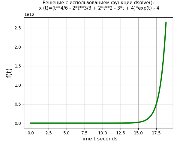
Program using the dsolve () function:

 from sympy import * import time import numpy as np import matplotlib.pyplot as plt start = time.time() var('t C1 C2 C3 C4') u = Function("u")(t) #   : de = Eq(u.diff(t, t, t, t) - 3*u.diff(t, t, t) + 3*u.diff(t, t) - u.diff(t), 4*t*exp(t)) #   : des = dsolve(de, u) #  : eq1 = des.rhs.subs(t, 0) eq2 = des.rhs.diff(t).subs(t, 0) eq3 = des.rhs.diff(t, t).subs(t, 0) eq4 = des.rhs.diff(t, t, t).subs(t, 0) #       : seq = solve([eq1, eq2-1, eq3-2, eq4-3], C1, C2, C3, C4) rez = des.rhs.subs([(C1, seq[C1]), (C2, seq[C2]), (C3, seq[C3]), (C4, seq[C4])]) def F(t): return rez f = lambdify(t, rez, 'numpy') x = np.linspace(0, 6*np.pi, 100) stop = time.time() print ('      dsolve(): %ss' % round((stop-start), 3)) plt.title('    dsolve():\n  (t)=%s\n' % rez, fontsize=11) plt.grid(True) plt.xlabel('Time t seconds', fontsize=12) plt.ylabel('f(t)', fontsize=16) plt.plot(x, f(x), color='#008000', linewidth=3) plt.show()

We get:

Time to solve the equation using the dsolve () function: 1.437 s

Program using Laplace transforms:

 from sympy import * import time import numpy as np import matplotlib.pyplot as plt start = time.time() var('s') var('t', positive=True) var('X', cls=Function) #  : x0 = 0 x01 = 0 x02 = 0 x03 = 0 #     : g = 4*t*exp(t) #   : Lg = laplace_transform(g, t, s, noconds=True) d4 = s**4*X(s) - s**3*x0 - s**2*x01 - s*x02 - x03 d3 = s**3*X(s) - s**2*x0 - s*x01 - x02 d2 = s**2*X(s) - s*x0 - x01 d1 = s*X(s) - x0 d0 = X(s) #     : d = factor(d4 - 3*d3 + 3*d2 - d1) de = Eq(d, Lg) #   : rez = solve(de, X(s))[0] #   : soln = collect(inverse_laplace_transform(rez, s, t), t) f = lambdify(t, soln, 'numpy') x = np.linspace(0, 6*np.pi, 100) stop = time.time() print ('      : %ss' % round((stop-start), 3)) plt.title('    :\n  (t)=%s\n' % soln, fontsize=11) plt.grid(True) plt.xlabel('t', fontsize=12) plt.ylabel('x(t)', fontsize=12) plt.plot(x, f(x), 'g', linewidth=2) plt.show()

We get:

The solution time of the equation using the Laplace transform: 3.274 s

So, the dsolve () function (1.437 s) solves the fourth order equation faster than the solution using the Laplace transform method (3.274 s) is more than doubled. However, it should be noted that the dsolve () function does not solve the system of differential equations of the second order, for example, when solving the system (6) using the dsolve () function, an error occurs:

 from sympy import* t = symbols('t') x, y = symbols('x, y', Function=True) eq = (Eq(Derivative(x(t), t, 2), -3*x(t) + y(t)), Eq(Derivative(y(t), t, 2), 2*x(t) - 2*y(t) + 40*sin(3*t))) rez = dsolve(eq) print (list(rez))

We get:

raiseNotImplementedError
NotImplementedError

This error means that the solution of the system of differential equations using the dsolve () function cannot be represented symbolically. Whereas with the help of the Laplace transforms we obtained a symbolic representation of the solution, and this proves the effectiveness of the proposed method.

Note.

To find the necessary method for solving differential equations using the dsolve () function, you need to use classify_ode (eq, f (x)) , for example:

 from sympy import * from IPython.display import * import matplotlib.pyplot as plt init_printing(use_latex=True) x = Symbol('x') f = Function('f') eq = Eq(f(x).diff(x, x) + f(x), 0) print (dsolve(eq, f(x))) print (classify_ode(eq, f(x))) eq = sin(x)*cos(f(x)) + cos(x)*sin(f(x))*f(x).diff(x) print (classify_ode(eq, f(x))) rez = dsolve(eq, hint='almost_linear_Integral') print (rez)

We get:

Eq (f (x), C1 * sin (x) + C2 * cos (x))
('nth_linear_constant_coeff_homogeneous', '2nd_power_series_ordinary')
('separable', '1st_exact', 'almost_linear', '1st_power_series', 'lie_group', 'separable_Integral', '1st_exact_Integral', 'almost_linear_Integral')
[Eq (f (x), -acos ((C1 + Integral (0, x)) * exp (-Integral (-tan (x), x))) + 2 * pi), Eq (f (x), acos ((C1 + Integral (0, x)) * exp (-Integral (-tan (x), x))))]

Thus, for the equation eq = Eq (f (x) .diff (x, x) + f (x), 0) , any method from the first list works:

nth_linear_constant_coeff_homogeneous,
2nd_power_series_ordinary

For the equation eq = sin (x) * cos (f (x)) + cos (x) * sin (f (x)) * f (x) .diff (x) , any method from the second list works:

separable, 1st_exact, almost_linear,
1st_power_series, lie_group, separable_Integral,
1st_exact_Integral, almost_linear_Integral

To use the selected method, the dsolve () function entry will look, for example:

 rez = dsolve(eq, hint='almost_linear_Integral')

Conclusion:

This article aimed to show how to use the SciPy and NumPy libraries using the example of solving linear ODE systems using an operator method. Thus, the methods of symbolic solution of linear differential equations and systems of equations by the Laplace method were considered. The analysis of the performance of this method and the methods implemented in the dsolve () function.

References:

Differential equations and boundary value problems: modeling and calculation using Mathematica, Maple and MATLAB. 3rd edition .: Trans. from English - M .: OOO “I.D. Williams ”, 2008. - 1104 pp., Il. - Paral. tit English
Using the inverse Laplace transform to analyze the dynamic links of control systems

Source: https://habr.com/ru/post/426041/

All Articles

Symbolic solution of linear differential equations and systems by the Laplace transform method using SymPy

The authorship history of the Laplace transform

The functions of the direct and inverse Laplace transform

Inverse Laplace transform on the example of determining the transition characteristics of regulators

Laplace transformation from higher order derivatives for solving the Cauchy problem

Method for solving linear differential equations and systems of equations based on Laplace transforms using the SymPy library

TAC functions

Conclusion:

More articles: