The principle of least action in analytical mechanics
Prehistory

The reason for this publication is an ambiguous article on the principle of least action (PND) , published on the resource a few days ago. It is ambiguous because its author in a popular form is trying to convey to the reader one of the fundamental principles of the mathematical description of nature, and this is partly possible for him. If it were not for one thing, lurking at the end of the publication. Under the spoiler is a full quote of this passage.
Not so simple
In fact, I was a little deceived, saying that the bodies always move so as to minimize the action. Although in many cases this is true, you can come up with situations in which the action is clearly not minimal.
')
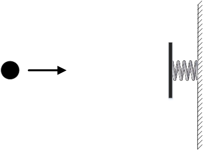
For example, take the ball and place it in the empty space. At some distance from him put an elastic wall. Suppose we want the ball to be in the same place after some time. Under such specified conditions, the ball can move in two different ways. First, he can just stay in place. Secondly, you can push it towards the wall. The ball will fly to the wall, bounce off of it and come back. It is clear that you can push it so fast that it returns at exactly the right time.
Both variants of the ball movement are possible, but the action in the second case will be more, because all this time the ball will move with non-zero kinetic energy.
How to save the principle of least action, so that it is fair in such situations? We will talk about this next time.
So what, in my opinion, is the problem?
The problem is that the author, citing this example, made a number of fundamental errors. It is aggravated by the fact that the planned second part, according to the author, will be based on these errors. Guided by the principle of filling the resource with reliable information, I have to speak in more detail about my position on this issue, and the format of comments for this is too small.
This article will talk about how mechanics are built on the basis of the HDPE, and will try to explain to the reader that the problem posed by the author of the cited publication is missing.
1. Definition of Hamilton action. Principle of least action
Hamilton action is called functional
S = i n t l i m i t s t 2 t 1 L l e f t ( m a t h b f q ( t ) , d o t m a t h b f q ( t ) r i g h t ) d t
Where
L left( mathbfq(t), dot mathbfq(t) right)=T left( mathbfq(t), dot mathbfq(t) right)− Pi( mathbfq)
- Lagrange function, for some mechanical system, in which (omitting the arguments in the following) T is the kinetic energy of the system; P - its potential energy; q (t) is the vector of generalized coordinates of this system, which is a function of time. at the same time, it is assumed that the times t 1 and t 2 are fixed.
Why functionality, but not function? Because a function, by definition, is a rule according to which one number from the domain (function argument) is assigned a different number from the domain. The functional differs in that the quality of its argument is not a number, but an entire function. In this case, it is the law of motion of the mechanical system q (t), determined at least over the time interval between t 1 and t 2 .
The perennial (and this is put it mildly!) Works of mechanical scientists (including the astounding Leonard Euler) made it possible to formulate
The principle of least action:
Mechanical system for which the Lagrange function is set L left( mathbfq(t), dot mathbfq(t) right) , moves in such a way that the law of its movement q (t) delivers a minimum to the functionalAlready from the very definition of PND, it follows that this principle leads to equations of motion only for a limited class of mechanical systems. For what? And let's see.S= int limitst2t1L left( mathbfq(t), dot mathbfq(t) right)dt to min
called the Hamilton action.
2. Limits of applicability of the principle of least action. Some definitions for the smallest
As follows from the definition, again, the Lagrange function, PND allows to obtain the equations of motion for mechanical systems, the force for which is determined solely by the potential energy. In order to figure out which systems we are talking about, we will give a few definitions, which, to save the volume of the article, I place under the spoiler
Elementary work force vecF on moving d vecs call a scalar equal to
dA= vecF cdotd vecs
Then, the total work of the force on moving a point along the path AB is a curvilinear integral
A= int limitsAB vecF cdotd vecs
The kinetic energy of the point T refers to the work that the forces applied to the point of mass m must perform in order to translate the point into motion with speed from the state of rest vecvCalculate the kinetic energy according to this definition. Let a point start moving from a state of rest under the action of forces applied to it. On the segment of the trajectory AB, it gains speed vecv . We calculate the work done by the forces applied to the point, which, according to the principle of independence of the action of the forces, will replace the resultant vecF
T=A= int limitsAB vecF cdotd vecs
In accordance with the second law of Newton
vecF=m veca=m fracd vecvdt
then
T= int limitsAB vecF cdotd vecs=m int limitsAB fracd vecvdt cdotd vecs=m int limitsAB vecv cdotd vecv
We compute the scalar product strictly standing under the integral sign, for which we differentiate in time the scalar product of the velocity vector of itself onto itself
fracddt( vecv cdot vecv)= fracd vecvdt cdot vecv+ vecv cdot fracd vecvdt=2 vecv cdot fracd vecvdt quad(1)
On the other hand,
vecv cdot vecv=v2
Differentiating this equality in time, we have
fracddt( vecv cdot vecv)= fracddt(v2)=2v fracdvdt quad(2)
Comparing (1) and (2) we conclude that
vecv cdotd vecv=vdv
Then, we calmly calculate the work, revealing the curvilinear integral through a definite one, taking the module of the velocity of a point at the beginning and at the end of the trajectory
T=m int limitsAB vecv cdotd vecv=m int limitsv0vdv= fracmv22
vecF= vecF(x,y,z) quad(3)
Let a point move in space along an arbitrary trajectory AB. Calculate what work the force will do (3)
A= int limitsAB vecF cdotd vecs= int limitsAB left(Fxdx+Fydy+Fzdz right)
Since the projection of force on the axes of coordinates depends solely on these very coordinates, you can always find the function
U=U(x,y,z)
such that
Fx= frac partialU partialx, quadFy= frac partialU partialy, quadFz= frac partialU partialz
Then, the expression for the work is converted to
A= int limitsAB left( frac partialU partialxdx+ frac partialU partialydy+ frac partialU partialzdz right)= int limitsUBUAdU=UB−UA
Where UA,UB - values of the function U (x, y, z) at points A and B, respectively. Thus, the work of the force under consideration does not depend on the trajectory of the point, but is determined only by the values of the function U at the beginning and at the end of the trajectory. Such a force is called a conservative force , and the corresponding function U (x, y, z) is a force function. It's obvious that vecF= nablaU , as well as the equality to zero of the work of a conservative force when moving along a closed trajectory. It is also said that the function U (x, y, z) in a space defines a force field.
Potential energy Pi= Pi(x,y,z) points in space with a given force field, call the work of external forces applied to it, which they perform when moving a point to a position given in coordinates (x, y, z) in space from some arbitrary position chosen as the starting point of the potential energy level .On the previously considered point trajectory, we choose an arbitrary point O lying between points A and B. We assume that the potential energy at point O is equal to zero. Then, according to the definition
PiA=−(UA−UO)
- the potential energy of a point at position A, and
PiB=−(UB−UO)
- potential energy of a point in position B. Considering all the above, we again calculate the work of potential forces on the displacement from point A to point B
AAB=AAO+AOB=UO−UA+UB−UO=(UO−UA)−(UO−UB)= PiA− PiB
Thus, the work of conservative forces is equal to the change in the potential energy of a point taken with the opposite sign
AAB= PiA− PiB=−( PiB− PiA)=− Delta Pi
and the choice of the level at which we consider the potential energy equal to zero does not affect the result at all. From this we can conclude that the reference level of potential energy can be chosen completely arbitrarily.
3. The concept of variations of generalized coordinates. Statement of the variational problem
So, we now consider a mechanical system moving under the action of potential forces, the position of which is uniquely given by the vector of generalized coordinates
mathbfq= left[q1,q2, dots,qs right]T quad(4)
where s is the number of degrees of freedom of the given system.
Actual, but not yet known to us , the law of motion of this system is determined by the dependence of the generalized coordinates (4) on time. Consider one of the generalized coordinates. qi=qi(t) assuming similar reasoning for all other coordinates.
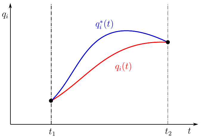
Figure 1. Real and detour movement of a mechanical system
In the figure, the dependence qi(t) depicted by a red curve. Choose two arbitrary fixed moments of time t 1 and t 2 , setting t 2 > t 1 . System position mathbfq1= mathbfq(t1) agree to call the initial position of the system, and mathbfq2= mathbfq(t2) - the final position of the system.
However, I once again insist that the following text be read carefully! Despite the fact that we set the initial and final position of the system, neither the first position nor the second is known to us in advance! As well as the unknown law of the movement of the system! These provisions are considered precisely as the initial and final position, regardless of specific values.
Further we assume that from the initial position to the final system can come in different ways, that is, the dependence mathbfq= mathbfq(t) can be any kinematically possible. The real motion of the system will exist in a single variant (red curve), the remaining kinematically possible variants will be called circumferential motions. mathbfq∗= mathbfq∗(t) (blue curve in the picture). Difference between real and roundabout traffic
deltaqi(t)=q∗i(t)−qi(t), quad foralli= overline1,s quad(5)
will be called isochronous variations of generalized coordinates
In this context, variations (5) should be understood as infinitesimal functions expressing the deviation of a roundabout motion from the real one. The small “delta” for the designation was not chosen randomly and underlines the fundamental difference between the variation and the differential of the function. The differential is the main linear part of the function increment, caused by the argument increment. In the case of variation, a change in the value of a function with a constant value of the argument is caused by a change in the type of the function itself! We do not vary the argument, in the role of which time plays, therefore the variation is called isochronous. We vary the rule according to which each value of time corresponds to a certain value of generalized coordinates!
In fact, we vary the law of motion according to which the system moves from the initial state to the final state. The initial and final states are determined by the actual law of motion, but I emphasize once again - we don’t know their specific values and can be any kinematically possible, we just assume that they exist and the system is guaranteed to move from one position to another! In the initial and final position of the system, we do not vary the law of motion; therefore, the variations of the generalized coordinates in the initial and final position are zero.
deltaqi(t1)= deltaqi(t2)=0, quad foralli= overline1,s quad(6)
Based on the principle of least action, the actual movement of the system should be such as to deliver a minimum of action functionality. Variation of coordinates causes a change in the action functional. A necessary condition for the achievement of an extremal value by a functional is that its variation is zero.
deltaS= delta int limitst2t1L(q1, dots,qs, dotq1, dots, dotqs)dt=0 quad(7)
4. The solution of the variational problem. Lagrange equations of the 2nd kind
We solve the variational problem we have set, for which we calculate the total variation of the action functional and equate it to zero
\ begin {align} \ delta S = & \ int \ limits_ {t_1} ^ {t2} \, L (q_1 + \ delta q_1, \ dots, q_s + \ delta q_s, \, \ dot q_1 + \ delta \ dot q_1, \ dots, \ dot q_s + \ delta \ dot q_s) \, dt - \\ & - \ int \ limits_ {t_1} ^ {t2} \, L (q_1, \ dots, q_s, \, \ dot q_1, \ dots, \ dot q_s) \, dt = 0 \ end {align}
We will drive everything under one integral, and since for variations all operations on infinitely small quantities are valid, we will transform this crocodile to the form
int limitst2t1 left[ sum limitssi=1 frac partialL partialqi deltaqi+ sum limitssi=1 frac partialL partial dotqi delta dotqi right]dt=0 quad(8)
Based on the definition of generalized speed
delta dotqi= fracd( deltaqi)dt
Then the expression (8) is converted to
int limitst2t1 left[ sum limitssi=1 frac partialL partialqi deltaqidt+ sum limitssi=1 frac partialL partial dotqid( deltaqi) right]=0
The second term is integrated in parts
sum limitssi=1 frac partialL partial dotqi deltaqi|t2t1+ int limitst2t1 left[ sum limitssi=1 frac partialL partialqi deltaqi− sum limitssi=1 fracddt left( frac partialL partial dotqi right) deltaqi right]dt=0 quad(10)
Based on condition (7), we have
sum limitssi=1 frac partialL partial dotqi deltaqi|t2t1=0
then, we get the equation
int limitst2t1 left[ sum limitssi=1 left( frac partialL partialqi− fracddt left( frac partialL partial dotqi right) right) deltaqi right]dt=0
With arbitrary limits of integration, the equality to zero of a certain integral is ensured by the equality to zero of the integrand
sum limitssi=1 left[ frac partialL partialqi− fracddt left( frac partialL partial dotqi right) right] deltaqi=0 quad(11)
Taking into account the fact that the variations of the generalized coordinates are independent, (11) is valid only if all coefficients are zero for variations, that is,
frac partialL partialqi− fracddt left( frac partialL partial dotqi right)=0, quad foralli= overline1,s
No one bothers us to multiply each of the equations by (-1) and get a more familiar record
fracddt left( frac partialL partial dotqi right)− frac partialL partialqi=0, quad foralli= overline1,s quad(12)
Equations (12) are the solution to the problem . And here at this point once again attention - the solution of a variational problem on the principle of least action, is not a function that delivers a minimum to the Hamilton action, but a system of differential equations that can be solved by solving such a function . In this case, this is the second-kind Lagrange differential equation written through the Lagrange function, that is, in the formulation for conservative mechanical systems.
And that's it, the principle of the smallest action ends , and the theory of ordinary differential equations begins, which, in particular, says that the solution of equation (12) is a vector function of the form
m a t h b f q = m a t h b f q ( t , C 1 , C 2 , d o t s , C 2 s )
where C 1 , ..., C 2s are arbitrary integration constants.
In this way
PND - a fundamental principle that allows to obtain the equations of motion of a system for which the Lagrange function is definedPoint! In the problems of analytical mechanics, the above calculations no longer need to be done, it is enough to use their result (12). The function that satisfies equation (12) is the law of motion of the system that satisfies the MHP.
5. The challenge with the ball and the wall
Now let us return to the problem with which everything began - about the one-dimensional motion of a ball near an absolutely elastic wall. Of course, for this problem one can obtain differential equations of motion. Since these are differential equations of motion, then any, I emphasize this, any solution to them delivers a minimum to the action functional, which means the HDPE is executed! The general solution of the equations of motion of a ball can be represented as a so-called phase portrait of the mechanical system under consideration. Here is the phase portrait
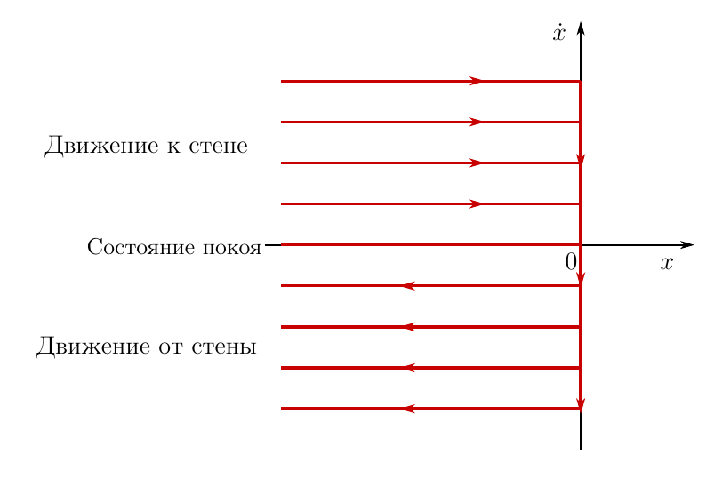
Figure 2. Phase portrait of the system in the problem with the ball
The coordinate of the ball is plotted along the horizontal axis, and the velocity projection onto the x axis is plotted along the vertical axis. It may seem strange, but this drawing reflects all possible phase trajectories of the ball, with any initial, or if you so wish, boundary conditions. In fact, there are infinitely many parallel lines on the graph; the drawing shows some of them and the direction of movement along the phase trajectory.
This is a general solution of the ball motion equation. Each of these phase trajectories provides a minimum of action functionality, which directly follows from the calculations performed above.
What does the author of the task? He says: the ball is at rest, and for the time from t A to t B the action is zero. If the ball is pushed to the wall, then for the same period of time the action will be longer, since the ball has a nonzero and constant kinetic energy. But why does the ball move to the wall, because at rest the action will be less? So PND is experiencing problems and does not work! But we will definitely solve it in the next article.
What the author says is nonsense. Why? Yes, because it compares the actions on different branches of the same real phase trajectory! Meanwhile, when using PND, the action is compared on the real trajectory and on the set of roundabout trajectories. That is, the action on the real trajectory is compared with the action on those trajectories that are not in nature, and never will be!
Unclear? I will explain even more intelligibly. Consider the state of rest. It is described by a branch of the phase portrait that coincides with the abscissa axis. Coordinate does not change over time. This is a real movement. And what kind of movement will be roundabout. Any other kinematically possible. For example, small oscillations of a ball near the rest position considered by us. The task allows the ball to oscillate along the x axis? Allows, then this movement is kinematically possible and can be considered as one of their devious
Why does the ball rest? Yes, because the action at rest, calculated on a fixed period of time from t A to t B , will be less than the action, with small fluctuations on the same period of time. It means that nature prefers rest to oscillations and any other “stirring” of the ball. In full compliance with the IPA.
Suppose we pushed the ball toward the wall. Suppose we pushed it as the author wants, at a speed selected from the boundary conditions, so that at time t B the ball is in the same position from which it started. The ball, at a constant speed, reaches the wall, bounces elastically and returns to the initial position at time t B , again at a constant speed. Ok, this is a real move. What movement will be one of the roundabouts? For example, if the ball moves to the wall and away from the wall at a rate varying with time. Such a movement is possible kinematically? Maybe. Why doesn't the speed of the ball change? Yes, because the effect on such a phase trajectory will have a minimum value, in comparison with any other option, where the speed depends on time.
That's all. Nothing such magic happens here. HDPE works without any problems.
Conclusions and wishes
PND is a fundamental law of nature. In particular, laws of mechanics, for example, differential equations of motion (12), follow from it. PND tells us that nature is structured in such a way that the equation of motion of a conservative mechanical system looks exactly like expression (12) and in no other way. More from him and is not required.
No need to invent problems where there are none.
Source: https://habr.com/ru/post/425771/
All Articles