Multi-armed gang problem - compare epsilon-greedy strategy and Thompson sampling
The task of the multi-armed gang
The multi-armed gang problem is one of the most basic tasks in the science of solutions. Namely, this is the problem of optimal allocation of resources under uncertainty conditions. The name "multi-armed gangster" came from the old slot machines, which were controlled with pens. These guns were nicknamed “bandits,” because after talking with them, people usually felt robbed. Now imagine that there are several such machines and the chance to win against different machines is different. Since we started to play with these machines, we want to determine which chance is higher and to use (exploit) this machine more often than others.
The problem is this: how is it most effective for us to understand which machine is best suited, and at the same time try out many possibilities in real time? This is not a theoretical problem, it is a problem that a business faces all the time. For example, a company has several options for messages that should be shown to users (messages include, for example, advertising, websites, images) so that the selected messages maximize a certain business task (conversion, clickability, etc.)
A typical way to solve this problem is to run A / B tests many times. Ie some weeks to show each of the options equally often, and then, based on statistical tests, decide which option is better. This method is suitable when there are few options, say 2 or 4. But when there are many options, this approach becomes ineffective - both for lost time and lost profits.
Where the lost time comes from should be easily understood. More options - more A / B tests are needed - more time is needed to make a decision. The loss of profits is not so obvious. Opportunity (opportunity cost) - the costs associated with the fact that instead of one action we did another, that is, to put it simply, this is what we lost by investing in A instead of B. Investing in B - and there is a loss of investment gain in A. Same with checking options. A / B tests should not be interrupted until they are over. This means that the experimenter does not know which option is better until testing has ended. However, it is still assumed that one option will be better than the other. This means that by extending the A / B tests, we do not show the best options to a sufficiently large number of visitors (although we don’t know which options are not the best), thereby losing our profit. This is the loss of profits from A / B testing. If there is only one A / B test, then perhaps the loss of profit is not great at all. A large number of A / V tests means that we have to show clients a lot of not the best options for a long time. It would be better if it were possible to quickly discard bad options in real time, and only then, when there are few options, use A / B tests for them.
Samplers or agents are ways to quickly test and optimize the distribution of variants. In this article, I will introduce you to Thompson sampling and its properties. I will also compare Thompson sampling with the epsilon-greedy algorithm — another popular option for the multiarmed gangster problem. Everything will be implemented in Python from scratch - all the code can be found here .
A brief dictionary of concepts
- Agent, sampler, gangster ( agent, sampler, bandit ) - an algorithm that makes decisions about which option to show.
- Option ( variant ) - a different version of the message that the visitor sees.
- Action ( action ) - the action that the algorithm chose (which option to show).
- Use ( exploit ) - to make a choice in order to maximize the total reward based on the available data.
- Explore, try ( explore ) - make a choice to better understand the return on investment for each option.
- Reward points ( score, reward ) - a business task, for example, conversion or clickability. For simplicity, we assume that it is distributed binomially and is either 1 or 0 - clicked or not.
- Environment - the context in which the agent works - options and their “payback” hidden for the user.
- Payback rate , success rate ( payout rate ) is a hidden variable equal to the probability of getting a score = 1, for each option it has its own. But the user does not see it.
- Trial ( trial ) - the user visits the page.
- Regret is the difference between what would be the best result of all the available options and what was the result of the option available on the current attempt. The less regret for actions already done, the better.
- Message ( message ) - a banner, a variant of the page, etc., the different versions of which we want to try.
- Sampling - the generation of a sample of a given distribution.
Explore and exploit
Agents are algorithms that look for an approach to choosing real-time solutions in order to achieve a balance between exploring the space of options and using the most optimal option. This balance is very important. The space of options must be explored in order to have an idea of which option is the best. If we first find this very optimal option, and then use it all the time, we maximize the total reward that is available to us from the environment. On the other hand, we also want to explore other possible options - what if they turn out to be better in the future, but we just don't know that yet? In other words, we want to insure against possible losses by trying to experiment a little with suboptimal options in order to clarify for themselves their payback. If their payback is actually higher, they can be shown more often. Another advantage of exploring options is that we can better understand not only the average payback, but also how roughly the payback is distributed, that is, we can better estimate the uncertainty.
The main problem, therefore, is to solve it - how best to get out of the dilemma between exploration and exploitation (exploration-exploitation tradeoff).
Epsilon-greedy algorithm (epsilon-greedy algorithm)
A typical way to get out of this dilemma is the epsilon-greedy algorithm. “Greedy” means exactly what you think. After a certain initial period, when we accidentally make attempts - say, 1000 times, the algorithm greedily chooses the best variant k in e percent of attempts. For example, if e = 0.05, the algorithm chooses the best option 95% of the time, and selects random attempts in the remaining 5% of the time. In fact, this is a fairly efficient algorithm, however, it may not sufficiently explore the space of options, and therefore, it is not good enough to evaluate which option is the best, to get stuck on a suboptimal version. Let's show in the code how this algorithm works.
But first, some dependencies. We need to define the environment. This is the context in which the algorithms will run. In this case, the context is very simple. He calls the agent so that the agent decides which action to choose, then the context then starts the action and returns the points received for it back to the agent (which somehow updates its state).
class Environment: def __init__(self, variants, payouts, n_trials, variance=False): self.variants = variants if variance: self.payouts = np.clip(payouts + np.random.normal(0, 0.04, size=len(variants)), 0, .2) else: self.payouts = payouts #self.payouts[5] = self.payouts[5] if i < n_trials/2 else 0.1 self.n_trials = n_trials self.total_reward = 0 self.n_k = len(variants) self.shape = (self.n_k, n_trials) def run(self, agent): """Run the simulation with the agent. agent must be a class with choose_k and update methods.""" for i in range(self.n_trials): # agent makes a choice x_chosen = agent.choose_k() # Environment returns reward reward = np.random.binomial(1, p=self.payouts[x_chosen]) # agent learns of reward agent.reward = reward # agent updates parameters based on the data agent.update() self.total_reward += reward agent.collect_data() return self.total_reward Points are distributed binomially with probability p, depending on the number of the action (just as they could be distributed and continuously, the essence would not have changed). I will also define the BaseSampler class — I just need it to store logs and various attributes.
class BaseSampler: def __init__(self, env, n_samples=None, n_learning=None, e=0.05): self.env = env self.shape = (env.n_k, n_samples) self.variants = env.variants self.n_trials = env.n_trials self.payouts = env.payouts self.ad_i = np.zeros(env.n_trials) self.r_i = np.zeros(env.n_trials) self.thetas = np.zeros(self.n_trials) self.regret_i = np.zeros(env.n_trials) self.thetaregret = np.zeros(self.n_trials) self.a = np.ones(env.n_k) self.b = np.ones(env.n_k) self.theta = np.zeros(env.n_k) self.data = None self.reward = 0 self.total_reward = 0 self.k = 0 self.i = 0 self.n_samples = n_samples self.n_learning = n_learning self.e = e self.ep = np.random.uniform(0, 1, size=env.n_trials) self.exploit = (1 - e) def collect_data(self): self.data = pd.DataFrame(dict(ad=self.ad_i, reward=self.r_i, regret=self.regret_i)) Below we define 10 options and payback for each. The best option is option 9 with a payback of 0.11%.
')
variants = [0, 1, 2, 3, 4, 5, 6, 7, 8, 9] payouts = [0.023, 0.03, 0.029, 0.001, 0.05, 0.06, 0.0234, 0.035, 0.01, 0.11] In order to make a start, we also define the class RandomSampler. This class is needed as a baseline model. He simply chooses an option on every attempt and does not update his parameters.
class RandomSampler(BaseSampler): def __init__(self, env): super().__init__(env) def choose_k(self): self.k = np.random.choice(self.variants) return self.k def update(self): # nothing to update #self.thetaregret[self.i] = self.thetaregret[self.i] #self.regret_i[self.i] = np.max(self.thetaregret) - self.theta[self.k] #self.thetas[self.i] = self.theta[self.k] self.thetaregret[self.i] = np.max(self.theta) - self.theta[self.k] self.a[self.k] += self.reward self.b[self.k] += 1 self.theta = self.a/self.b self.ad_i[self.i] = self.k self.r_i[self.i] = self.reward self.i += 1 Other models have the following structure. All have methods choose_k and update. choose_k implements the method by which the agent chooses an option. update updates the parameters of the agent - this method describes how the ability of the agent to select an option changes (for RandomSampler this possibility does not change at all). We run the agent in the environment using the following pattern.
en0 = Environment(machines, payouts, n_trials=10000) rs = RandomSampler(env=en0) en0.run(agent=rs) The essence of the epsilon-greedy algorithm is as follows.
- Randomly select k for n attempts.
- For each attempt to evaluate the gain for each option.
- After all n attempts:
- With a probability of 1– e, choose the k with the highest gain;
- With probability e, choose K randomly.
Epsilon Greedy Code:
class eGreedy(BaseSampler): def __init__(self, env, n_learning, e): super().__init__(env, n_learning, e) def choose_k(self): # e% of the time take a random draw from machines # random k for n learning trials, then the machine with highest theta self.k = np.random.choice(self.variants) if self.i < self.n_learning else np.argmax(self.theta) # with 1 - e probability take a random sample (explore) otherwise exploit self.k = np.random.choice(self.variants) if self.ep[self.i] > self.exploit else self.k return self.k # every 100 trials update the successes # update the count of successes for the chosen machine def update(self): # update the probability of payout for each machine self.a[self.k] += self.reward self.b[self.k] += 1 self.theta = self.a/self.b #self.total_reward += self.reward #self.regret_i[self.i] = np.max(self.theta) - self.theta[self.k] #self.thetaregret[self.i] = self.thetaregret[self.i] self.thetas[self.i] = self.theta[self.k] self.thetaregret[self.i] = np.max(self.thetas) - self.theta[self.k] self.ad_i[self.i] = self.k self.r_i[self.i] = self.reward self.i += 1 Below on the graph you can see the results of a purely random sampling, that is, in other words, there is no model here. The graph shows what choice the algorithm made on each attempt, if there were 10 thousand attempts. The algorithm only tries, but does not learn. He scored 418 points in total.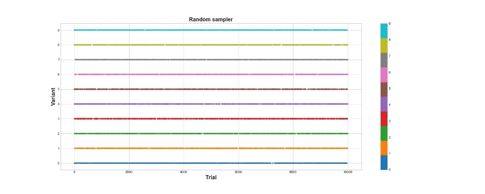
Let's see how the epsilon-greedy algorithm behaves in the same environment. Let's run the algorithm for 10 thousand attempts with e = 0.1 and n_learning = 500 (the agent simply tries the first 500 attempts, then tries it with probability e = 0.1). We will evaluate the algorithm according to the total number of points it collects in the environment.
en1 = Environment(machines, payouts, n_trials) eg = eGreedy(env=en1, n_learning=500, e=0.1) en1.run(agent=eg) 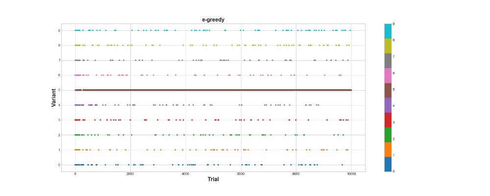
Epsilon-greedy algorithm scored 788 points, almost 2 times better than a random algorithm - super! The second graph explains this algorithm quite well. We see that for the first 500 steps, the actions are distributed approximately evenly and K is chosen randomly. However, then it begins to exploit strongly option 5 - this is a pretty strong option, but not the best. We also see that the agent still chooses randomly 10% of the time.
This is pretty cool - we wrote just a few lines of code, and now we already have a fairly powerful algorithm that can explore the space of options and make it close to the optimal solution. On the other hand, the algorithm did not find the best option. Yes, we can increase the number of steps for training, but in this way we will spend even more time on a random search, further worsening the final result. Also, randomness is sewn into this process by default - the best algorithm may never be found.
Later, I will run each of the algorithms many times so that we can compare them relative to each other. But for now, let's deal with Thompson sampling and test it in the same environment.
Thompson sampling
Thompson sampling is fundamentally different from the epsilon-greedy algorithm in three main points:
- It is not greedy.
- It makes attempts in a more intricate way.
- It is Bayesian.
The main point is point 3, points 1 and 2 follow from it.
The essence of the algorithm is as follows:
- Set the initial Beta distribution between 0 and 1 for the payback of each option.
- To sample the options from this distribution, select the maximum parameter Theta.
- Choose a variant of k, which would be associated with the biggest theta.
- See how many points scored, update the distribution parameters.
You can read more about beta distribution here .
And about its use in Python - here .
Algorithm code:
class ThompsonSampler(BaseSampler): def __init__(self, env): super().__init__(env) def choose_k(self): # sample from posterior (this is the thompson sampling approach) # this leads to more exploration because machines with > uncertainty can then be selected as the machine self.theta = np.random.beta(self.a, self.b) # select machine with highest posterior p of payout self.k = self.variants[np.argmax(self.theta)] #self.k = np.argmax(self.a/(self.a + self.b)) return self.k def update(self): #update dist (a, b) = (a, b) + (r, 1 - r) self.a[self.k] += self.reward self.b[self.k] += 1 - self.reward # ie only increment b when it's a swing and a miss. 1 - 0 = 1, 1 - 1 = 0 #self.thetaregret[self.i] = self.thetaregret[self.i] #self.regret_i[self.i] = np.max(self.theta) - self.theta[self.k] self.thetas[self.i] = self.theta[self.k] self.thetaregret[self.i] = np.max(self.thetas) - self.theta[self.k] self.ad_i[self.i] = self.k self.r_i[self.i] = self.reward self.i += 1 The formal writing of the algorithm is as follows.
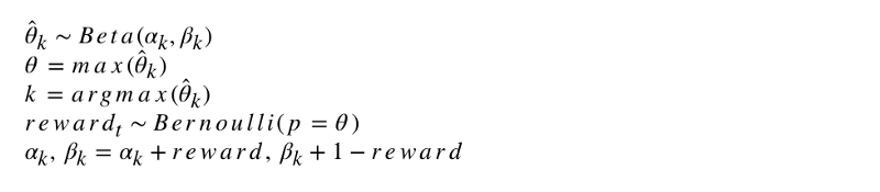
Let's program this algorithm. Like other agents, ThompsonSampler inherits from BaseSampler and defines its own choose_k and update methods. Now let's launch our new agent.
en2 = Environment(machines, payouts, n_trials) tsa = ThompsonSampler(env=en2) en2.run(agent=tsa) 
As you can see, he scored more than the epsilon-greedy algorithm. Super! Let's look at the schedule for the selection of attempts. It shows two interesting things. First, the agent correctly discovered the best option (option 9) and used it to its fullest. Secondly, the agent used other options, but in a more cunning way - after about 1000 attempts, the agent, besides the main option, mainly used the strongest options among the rest. In other words, he chose not at random, but more competently.
Why does this work? Everything is simple - the uncertainty in the posterior distribution of the expected benefits for each option means that each option is chosen with a probability approximately proportional to its form, determined by the alpha and beta parameters. In other words, at each attempt, Thompson sampling triggers a variant according to the posterior probability that the maximum benefit is from him. Roughly speaking, having an uncertainty information distribution, the agent decides when to explore the environment and when to use the information. For example, a weak version with high posterior ambiguity can pay off most for a given attempt. But for the majority of attempts, the stronger his posterior distribution, the greater his average and the smaller his standard deviation, and therefore, the greater the chances of choosing it.
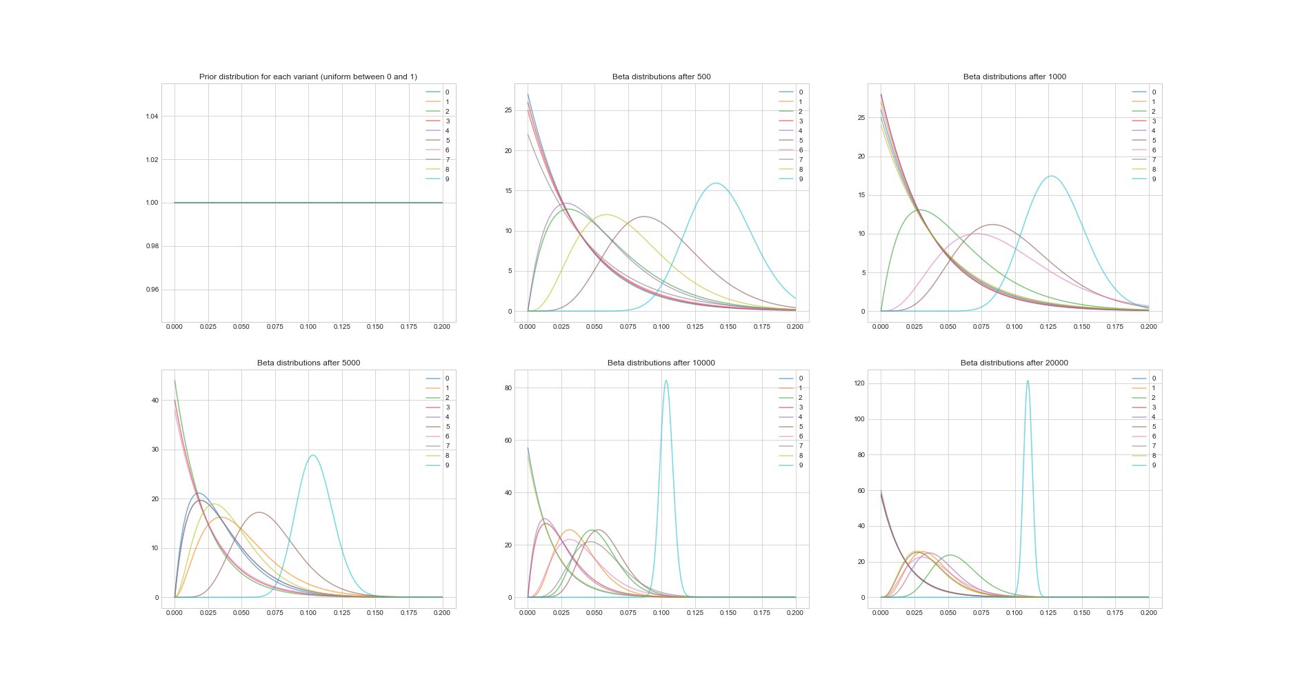
Another remarkable property of the Thompson algorithm is: since it is Bayesian, we can estimate its parameters by estimating the uncertainty in the estimated payback for each option. The graph below shows posterior distributions at 6 different points and in 20,000 attempts. You see, as the distributions gradually begin to converge to the option with the best payback.
Now compare all 3 agents on 100 simulations. Simulation 1 is an agent launch on 10,000 attempts.
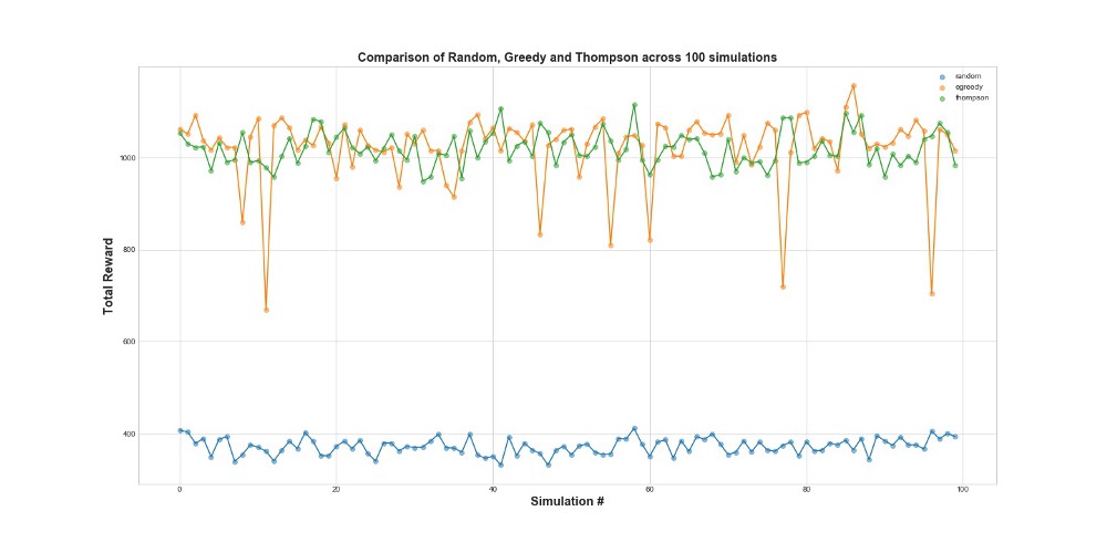
As can be seen from the graph, both the epsilon-greedy strategy and Thompson sampling work much better than random sampling. You may be surprised that epsilon-greedy strategy and Thompson sampling are actually comparable in terms of their performance. Epsilon-greedy strategy can be very effective, but it is more risky, because it can get stuck on a suboptimal version - this can be seen on the failures in the graph. And Thompson sampling cannot, because it makes the choice in the space of options in a more complicated way.
Regret
Another way to evaluate how well the algorithm works is to evaluate regret (regret). Roughly speaking, the smaller it is, in relation to actions already done, the better. Below is a graph of total regret and regret for the mistake. Once again - the less regret, the better.
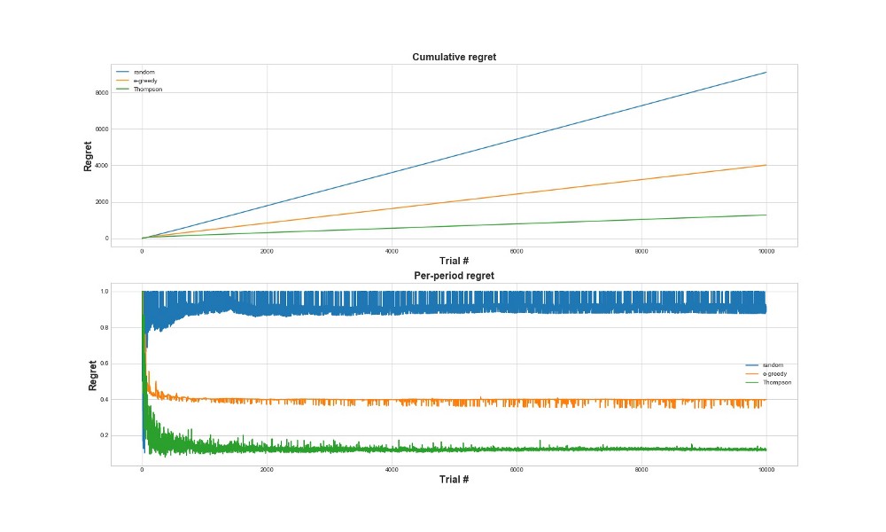
In the upper graph, we see a cumulative regret, and in the bottom a regret at the attempt. As can be seen from the graphs, the Thompson sampling converges to minimal regret much faster than the epsilon-greedy strategy. And it converges to a lower level. With Thomson sampling, the agent regrets less because he can better discover the best option and better try the most promising options - so Thomson sampling is particularly well suited to more advanced use cases, such as statistical models or neural network to select k.
findings
This is a fairly long technical post. To summarize, we can use quite complex sampling methods, if we have a lot of options that we want to test in real time. One of Thompson's very good sampling features is that it balances usage and research in a rather tricky way. That is, we can allow it to optimize the distribution of solution options in real time. These are cool algorithms, and they should be more useful for business than A / B tests.
Important! Thompson sampling does not mean that you do not need to do A / B tests. Usually, with its help, the best options are found, and then A / B tests are done on them.
Source: https://habr.com/ru/post/425619/
All Articles