Game Theory: Decision Making with Kotlin Examples
Game theory is a mathematical discipline that considers the modeling of actions of players who have a goal, which is to choose the optimal strategies of behavior in conditions of conflict. On Habré, this topic has already been covered , but today we will talk about some of its aspects in more detail and consider examples on Kotlin.
So, a strategy is a set of rules that determine the choice of a course of action for each personal move, depending on the situation. The optimal player strategy is a strategy that provides the best position in this game, i.e. maximum winnings If the game is repeated several times and contains, besides personal, random moves, then the optimal strategy provides the maximum average gain.
The task of game theory is to identify the optimal strategies of players. The main assumption, on the basis of which the optimal strategies are found, is that the opponent (or opponents) is no less intelligent than the player himself, and does everything to achieve his goal. Relying on a sensible adversary is only one of the potential positions in a conflict, but in the theory of games, it is she who is the basis.
There are games with nature in which there is only one participant maximizing their profits. Games with nature are mathematical models in which the choice of decision depends on objective reality. For example, customer demand, state of nature, etc. “Nature” is a generalized concept of an adversary who does not pursue his own goals. In this case, several criteria are used to select the optimal strategy.
There are two types of tasks in games with nature:
')
Briefly about these criteria described here .
Now we will consider the decision criteria in pure strategies, and at the end of the article we will solve the game in mixed strategies by an analytical method.
All decision criteria, we will analyze the end-to-end example. The task is this: the farmer needs to determine in what proportions to sow his field with three crops, if the yield of these crops, and, therefore, profit, depend on what summer will be: cool and rainy, normal, or hot and dry. The farmer calculated the net profit from 1 hectare from different crops depending on the weather. The game is determined by the following matrix:

Further we will present this matrix in the form of strategies:
Looking for the optimal strategy we denote uopt . We will solve the game using the criteria of Wald, optimism, pessimism, Savage and Hurwitz under conditions of uncertainty and the criteria of Bayes and Laplace under conditions of risk.
As mentioned above, examples will be on Kotlin. I note that there are generally solutions like Gambit (written in C), Axelrod and PyNFG (written in Python), but we will ride our own bike, assembled on the knee, just to poke a little stylish, trendy and youth programming language.
In order to programmatically implement the solution of the game, we will create several classes. First, we need a class that allows us to describe a row or column of the game matrix. The class is extremely simple and contains a list of possible values (alternatives or states of nature) and the corresponding name. The
The game matrix contains information about alternatives and states of nature. In addition, it implements some methods, such as finding the dominant set and the net price of the game.
We describe the interface that meets the criteria
Decision making under uncertainty implies that the player is not opposed by a reasonable opponent.
In the Wald criterion, the worst possible outcome is maximized:
Using the criterion insures against the worst result, but the price of such a strategy is the loss of the opportunity to get the best possible result.
Consider an example. For strategies U1=(0,2,5),U2=(2,3,1),U3=(4,3,−1) find the minimums and get the next three S=(0,1,−1) . The maximum for the indicated three will be the value 1, therefore, according to the Wald criterion, the winning strategy is the strategy U2=(2,3,1) corresponding to planting culture 2.
Software implementation of the Wald criterion is simple:
For greater clarity, for the first time I will show how the solution would look like a test:
It is not difficult to guess that for other criteria the difference will be only in the creation of the object
When using the optimist criterion, the player chooses a solution that gives the best result, while the optimist assumes that the conditions of the game will be most favorable for him:
An optimist's strategy can lead to negative consequences when the maximum supply coincides with the minimum demand — a firm may suffer losses when writing off unsold products. At the same time, the strategy of the optimist has a certain meaning, for example, there is no need to worry about unsatisfied customers, since any possible demand is always satisfied, so there is no need to maintain the location of customers. If the maximum demand is realized, the strategy of the optimist allows you to get the maximum utility at the time, as other strategies will lead to lost profits. This gives certain competitive advantages.
Consider an example. For strategies U1=(0,2,5),U2=(2,3,1),U3=(4,3,−1) find the maximum and get the next three S=(5,3,4) . The maximum for the indicated three will be 5, therefore, according to the criterion of optimism, the winning strategy is the strategy U1=(0,2,5) corresponding to planting culture 1.
The implementation of the optimism criterion hardly differs from the Wald criterion:
This criterion is designed to select the smallest element of the game matrix from its minimum possible elements:
The criterion of pessimism suggests that developments will be unfavorable for the decision maker. When using this criterion, the decision maker is guided by the possible loss of control over the situation, therefore, he tries to eliminate potential risks by choosing the option with the minimum yield.
Consider an example. For strategies U1=(0,2,5),U2=(2,3,1),U3=(4,3,−1) find the minimum and get the next three S=(0,1,−1) . The minimum for the specified three will be -1, therefore, according to the criterion of pessimism, the winning strategy is the strategy U3=(4.3,−1) corresponding to planting culture 3.
After getting acquainted with the Wald and optimism criteria, I think it is easy to guess what the class of pessimism criterion will look like:
The Savage Criterion (a regretting pessimist criterion) involves minimizing the greatest lost profits, in other words, the greatest regrets for lost profits are minimized:
In this case, S is a regret matrix.
The optimal solution according to the Savage criterion should give the least regret of the regrets found at the previous step. The solution corresponding to the found utility will be optimal.
The peculiarities of the solution obtained include the guaranteed absence of the greatest disappointments and the guaranteed reduction of the maximum possible gains of other players.
Consider an example. For strategies U1=(0,2,5),U2=(2,3,1),U3=(4,3,−1) we will make a regret matrix:
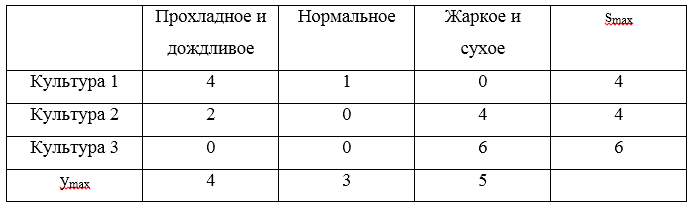
Three of maximum regrets S=(4,4,6) . The minimum value of these risks will be 4, which corresponds to the strategies U1 and U2 .
To program the Savage criterion is a little more difficult:
The Hurwitz criterion is a regulated compromise between extreme pessimism and complete optimism:
A (0) is the strategy of the extreme pessimist, A (k) is the strategy of a complete optimist, gamma=1 - set value of weight coefficient: 0 leq gamma leq1 ; gamma=0 - extreme pessimism, gamma=1 - complete optimism.
With a small number of discrete strategies, setting the desired value of the weighting factor gamma and then round the result to the nearest possible value, taking into account the performed sampling.
Consider an example. For strategies U1=(0,2,5),U2=(2,3,1),U3=(4,3,−1) . We assume that the coefficient of optimism gamma=$0. . Now we will make the table:
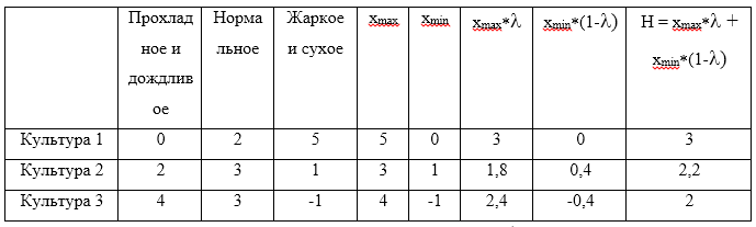
The maximum value of the calculated H will be 3, which corresponds to the strategy U1 .
The implementation of the Hurwitz criterion is already more voluminous:
Decision making methods can rely on decision criteria under risk conditions if the following conditions are met:
If the decision is made under risk, then the cost of alternative solutions are described by probability distributions. In this regard, the decision is based on the use of the criterion of the expected value, according to which alternative solutions are compared in terms of maximizing the expected profit or minimizing the expected costs.
The expected value criterion can be reduced to either maximizing the expected (average) profit, or minimizing the expected costs. In this case, it is assumed that the profit (cost) associated with each alternative solution is a random variable.
The formulation of such tasks is usually the following: a person chooses some actions in a situation where random events affect the outcome of actions. But the player has some knowledge about the probabilities of these events and can calculate the most advantageous set and sequence of his actions.
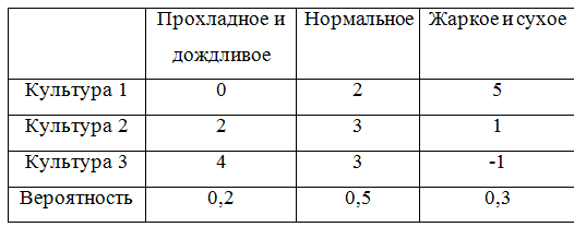
So that you can continue to give examples, let's add the game matrix with probabilities:
In order to take into account the probabilities will have to alter a little class that describes the game matrix. It turned out, in truth, not very elegant, but oh well.
Bayes criterion (expectation criterion) is used in decision making under risk as a strategy assessment. ui the mathematical expectation of the corresponding random variable appears. In accordance with this rule, the optimal strategy of the player uopt is found from the condition:
In other words, an indicator of the strategy’s inefficiency ui according to the Bayes criterion with respect to risks, the average value (expectation) of the risks of the i-th row of the matrix is U whose probabilities coincide with the probabilities of nature. Then the optimal among the pure strategies for the Bayes criterion regarding risks is the strategy uopt which has minimal inefficiency, that is, minimal average risk. The Bayes criterion is equivalent to gains and risks, i.e. if strategy uopt is optimal for the Bayes criterion for winnings, it is optimal for the Bayes criterion for risks, and vice versa.
Let us turn to an example and calculate the mathematical expectations:
The maximum expected value is M1 therefore, the winning strategy is strategy U1 .
Software implementation of the Bayesian criterion:
The Laplace criterion represents a simplified maximization of the expectation of utility when the assumption of equal probability of demand levels is true, which eliminates the need to collect real statistics.
In the general case, when using the Laplace criterion, the matrix of expected utilities and the optimal criterion are determined as follows:
Consider an example of decision making based on the Laplace criterion. Calculate the average for each strategy:
Thus, the winning strategy is the strategy U1 .
Software implementation of the Laplace criterion:
The analytical method allows to solve the game in mixed strategies. In order to formulate an algorithm for finding the solution of a game by an analytical method, consider some additional concepts.
Strategy Ui dominated by strategy Ui−1 , If everyone u1..n inUi gequ1..n inUi−1 .In other words, if in a certain row of the payment matrix all elements are greater than or equal to the corresponding elements of another row, then the first row dominates the second and is called the dominant row. And also if in some column of the payment matrix all elements are less or equal to the corresponding elements of another column, then the first column dominates the second one and is called the dominant column.
The bottom price of the game is calledα = m a x i m i n j u i i .
The top price of the game is called β = m i n j m a x i u i j .
Now we can formulate an algorithm for solving a game using the analytical method:
In order to give an example, you must provide a class that describes the solution.
And the class that performs the solution simplex method. Since I don’t understand mathematics, I used the ready implementation from Apache Commons Math
Now we will execute the decision by an analytical method. For clarity, we take another game matrix:
There is a dominant set in this matrix:
( 2 4 6 2 )
Game solution ( 0 , 33 ; 0 , 67 ; 0 ) with the price of the game equal to 3.33
I hope this article will be useful to those who need a first approximation with the decision of games with nature. Instead of conclusions link to GitHub .
I would be grateful for the constructive feedback!
So, a strategy is a set of rules that determine the choice of a course of action for each personal move, depending on the situation. The optimal player strategy is a strategy that provides the best position in this game, i.e. maximum winnings If the game is repeated several times and contains, besides personal, random moves, then the optimal strategy provides the maximum average gain.
The task of game theory is to identify the optimal strategies of players. The main assumption, on the basis of which the optimal strategies are found, is that the opponent (or opponents) is no less intelligent than the player himself, and does everything to achieve his goal. Relying on a sensible adversary is only one of the potential positions in a conflict, but in the theory of games, it is she who is the basis.
There are games with nature in which there is only one participant maximizing their profits. Games with nature are mathematical models in which the choice of decision depends on objective reality. For example, customer demand, state of nature, etc. “Nature” is a generalized concept of an adversary who does not pursue his own goals. In this case, several criteria are used to select the optimal strategy.
There are two types of tasks in games with nature:
')
- the problem of making decisions under risk conditions, when the probabilities with which nature assumes each of the possible states are known;
- decision-making problems in conditions of uncertainty, when there is no possibility to obtain information about the probabilities of the appearance of states of nature.
Briefly about these criteria described here .
Now we will consider the decision criteria in pure strategies, and at the end of the article we will solve the game in mixed strategies by an analytical method.
Clause
I am not an expert in game theory, and in this work I used Kotlin for the first time. However, I decided to share my results. If you notice errors in the article or want to give advice, please in PM.
Formulation of the problem
All decision criteria, we will analyze the end-to-end example. The task is this: the farmer needs to determine in what proportions to sow his field with three crops, if the yield of these crops, and, therefore, profit, depend on what summer will be: cool and rainy, normal, or hot and dry. The farmer calculated the net profit from 1 hectare from different crops depending on the weather. The game is determined by the following matrix:
Further we will present this matrix in the form of strategies:
U1=(0,2,5),U2=(2,3,1),U3=(4,3,−1)
Looking for the optimal strategy we denote uopt . We will solve the game using the criteria of Wald, optimism, pessimism, Savage and Hurwitz under conditions of uncertainty and the criteria of Bayes and Laplace under conditions of risk.
As mentioned above, examples will be on Kotlin. I note that there are generally solutions like Gambit (written in C), Axelrod and PyNFG (written in Python), but we will ride our own bike, assembled on the knee, just to poke a little stylish, trendy and youth programming language.
In order to programmatically implement the solution of the game, we will create several classes. First, we need a class that allows us to describe a row or column of the game matrix. The class is extremely simple and contains a list of possible values (alternatives or states of nature) and the corresponding name. The
key field will be used for identification, as well as for comparison, and the comparison will be needed when implementing dominance.Row or column of the game matrix
import java.text.DecimalFormat import java.text.NumberFormat open class GameVector(name: String, values: List<Double>, key: Int = -1) : Comparable<GameVector> { val name: String val values: List<Double> val key: Int private val formatter:NumberFormat = DecimalFormat("#0.00") init { this.name = name; this.values = values; this.key = key; } public fun max(): Double? { return values.max(); } public fun min(): Double? { return values.min(); } override fun toString(): String{ return name + ": " + values .map { v -> formatter.format(v) } .reduce( {f1: String, f2: String -> "$f1 $f2"}) } override fun compareTo(other: GameVector): Int { var compare = 0 if (this.key == other.key){ return compare } var great = true for (i in 0..this.values.lastIndex){ great = great && this.values[i] >= other.values[i] } if (great){ compare = 1 }else{ var less = true for (i in 0..this.values.lastIndex){ less = less && this.values[i] <= other.values[i] } if (less){ compare = -1 } } return compare } } The game matrix contains information about alternatives and states of nature. In addition, it implements some methods, such as finding the dominant set and the net price of the game.
Game matrix
open class GameMatrix(matrix: List<List<Double>>, alternativeNames: List<String>, natureStateNames: List<String>) { val matrix: List<List<Double>> val alternativeNames: List<String> val natureStateNames: List<String> val alternatives: List<GameVector> val natureStates: List<GameVector> init { this.matrix = matrix; this.alternativeNames = alternativeNames this.natureStateNames = natureStateNames var alts: MutableList<GameVector> = mutableListOf() for (i in 0..matrix.lastIndex) { val currAlternative = alternativeNames[i] val gameVector = GameVector(currAlternative, matrix[i], i) alts.add(gameVector) } alternatives = alts.toList() var nss: MutableList<GameVector> = mutableListOf() val lastIndex = matrix[0].lastIndex // , for (j in 0..lastIndex) { val currState = natureStateNames[j] var states: MutableList<Double> = mutableListOf() for (i in 0..matrix.lastIndex) { states.add(matrix[i][j]) } val gameVector = GameVector(currState, states.toList(), j) nss.add(gameVector) } natureStates = nss.toList() } open fun change (i : Int, j : Int, value : Double) : GameMatrix{ var mml = this.matrix.toMutableList() var rowi = mml[i].toMutableList() rowi.set(j, value) mml.set(i, rowi) return GameMatrix(mml.toList(), alternativeNames, natureStateNames) } open fun changeAlternativeName (i : Int, value : String) : GameMatrix{ var list = alternativeNames.toMutableList() list.set(i, value) return GameMatrix(matrix, list.toList(), natureStateNames) } open fun changeNatureStateName (j : Int, value : String) : GameMatrix{ var list = natureStateNames.toMutableList() list.set(j, value) return GameMatrix(matrix, alternativeNames, list.toList()) } fun size() : Pair<Int, Int>{ return Pair(alternatives.size, natureStates.size) } override fun toString(): String { return " :\n" + natureStateNames.reduce { n1: String, n2: String -> "$n1;\n$n2" } + "\n :\n" + alternatives .map { a: GameVector -> a.toString() } .reduce { a1: String, a2: String -> "$a1;\n$a2" } } protected fun dominateSet(gvl: List<GameVector>, list: MutableList<String>, dvv: Int) : MutableSet<GameVector>{ var dSet: MutableSet<GameVector> = mutableSetOf() for (gv in gvl){ for (gvv in gvl){ if (!dSet.contains(gv) && !dSet.contains(gvv)) { if (gv.compareTo(gvv) == dvv) { dSet.add(gv) list.add("[$gvv] [$gv]") } } } } return dSet } open fun newMatrix(dCol: MutableSet<GameVector>, dRow: MutableSet<GameVector>) : GameMatrix{ var result: MutableList<MutableList<Double>> = mutableListOf() var ralternativeNames: MutableList<String> = mutableListOf() var rnatureStateNames: MutableList<String> = mutableListOf() val dIndex = dCol.map { c -> c.key }.toList() for (i in 0 .. natureStateNames.lastIndex){ if (!dIndex.contains(i)){ rnatureStateNames.add(natureStateNames[i]) } } for (gv in this.alternatives){ if (!dRow.contains(gv)){ var nr: MutableList<Double> = mutableListOf() for (i in 0 .. gv.values.lastIndex){ if (!dIndex.contains(i)){ nr.add(gv.values[i]) } } result.add(nr) ralternativeNames.add(gv.name) } } val rlist = result.map { r -> r.toList() }.toList() return GameMatrix(rlist, ralternativeNames.toList(), rnatureStateNames.toList()) } fun dominateMatrix(): Pair<GameMatrix, List<String>>{ var list: MutableList<String> = mutableListOf() var dCol: MutableSet<GameVector> = dominateSet(this.natureStates, list, 1) var dRow: MutableSet<GameVector> = dominateSet(this.alternatives, list, -1) val newMatrix = newMatrix(dCol, dRow) var ddgm = Pair(newMatrix, list.toList()) val ret = iterate(ddgm, list) return ret; } protected fun iterate(ddgm: Pair<GameMatrix, List<String>>, list: MutableList<String>) : Pair<GameMatrix, List<String>>{ var dgm = this var lddgm = ddgm while (dgm.size() != lddgm.first.size()){ dgm = lddgm.first list.addAll(lddgm.second) lddgm = dgm.dominateMatrix() } return Pair(dgm,list.toList().distinct()) } fun minClearPrice(): Double{ val map: List<Double> = this.alternatives.map { a -> a?.min() ?: 0.0 } return map?.max() ?: 0.0 } fun maxClearPrice(): Double{ val map: List<Double> = this.natureStates.map { a -> a?.max() ?: 0.0 } return map?.min() ?: 0.0 } fun existsClearStrategy() : Boolean{ return minClearPrice() >= maxClearPrice() } } We describe the interface that meets the criteria
Criterion
interface ICriteria { fun optimum(): List<GameVector> } Decision making under uncertainty
Decision making under uncertainty implies that the player is not opposed by a reasonable opponent.
Wald Criterion
In the Wald criterion, the worst possible outcome is maximized:
uopt=maximinj[U]
Using the criterion insures against the worst result, but the price of such a strategy is the loss of the opportunity to get the best possible result.
Consider an example. For strategies U1=(0,2,5),U2=(2,3,1),U3=(4,3,−1) find the minimums and get the next three S=(0,1,−1) . The maximum for the indicated three will be the value 1, therefore, according to the Wald criterion, the winning strategy is the strategy U2=(2,3,1) corresponding to planting culture 2.
Software implementation of the Wald criterion is simple:
class WaldCriteria(gameMatrix : GameMatrix) : ICriteria { val gameMatrix: GameMatrix init{ this.gameMatrix = gameMatrix } override fun optimum(): List<GameVector> { val mins = gameMatrix.alternatives.map { a -> Pair(a, a.min()) } val max = mins.maxWith( Comparator { o1, o2 -> o1.second!!.compareTo(o2.second!!)}) return mins .filter { m -> m.second == max!!.second } .map { m -> m.first } } } For greater clarity, for the first time I will show how the solution would look like a test:
Test
private fun matrix(): GameMatrix { val alternativeNames: List<String> = listOf(" 1", " 2", " 3") val natureStateNames: List<String> = listOf(" ", "", " ") val matrix: List<List<Double>> = listOf( listOf(0.0, 2.0, 5.0), listOf(2.0, 3.0, 1.0), listOf(4.0, 3.0, -1.0) ) val gm = GameMatrix(matrix, alternativeNames, natureStateNames) return gm; } } private fun testCriteria(gameMatrix: GameMatrix, criteria: ICriteria, name: String){ println(gameMatrix.toString()) val optimum = criteria.optimum() println("$name. : ") optimum.forEach { o -> println(o.toString()) } } @Test fun testWaldCriteria() { val matrix = matrix(); val criteria = WaldCriteria(matrix) testCriteria(matrix, criteria, " ") } It is not difficult to guess that for other criteria the difference will be only in the creation of the object
criteria .Optimism criterion
When using the optimist criterion, the player chooses a solution that gives the best result, while the optimist assumes that the conditions of the game will be most favorable for him:
uopt=maximaxj[U]
An optimist's strategy can lead to negative consequences when the maximum supply coincides with the minimum demand — a firm may suffer losses when writing off unsold products. At the same time, the strategy of the optimist has a certain meaning, for example, there is no need to worry about unsatisfied customers, since any possible demand is always satisfied, so there is no need to maintain the location of customers. If the maximum demand is realized, the strategy of the optimist allows you to get the maximum utility at the time, as other strategies will lead to lost profits. This gives certain competitive advantages.
Consider an example. For strategies U1=(0,2,5),U2=(2,3,1),U3=(4,3,−1) find the maximum and get the next three S=(5,3,4) . The maximum for the indicated three will be 5, therefore, according to the criterion of optimism, the winning strategy is the strategy U1=(0,2,5) corresponding to planting culture 1.
The implementation of the optimism criterion hardly differs from the Wald criterion:
class WaldCriteria(gameMatrix : GameMatrix) : ICriteria { val gameMatrix: GameMatrix init{ this.gameMatrix = gameMatrix } override fun optimum(): List<GameVector> { val mins = gameMatrix.alternatives.map { a -> Pair(a, a.min()) } val max = mins.maxWith( Comparator { o1, o2 -> o1.second!!.compareTo(o2.second!!)}) return mins .filter { m -> m.second == max!!.second } .map { m -> m.first } } } Pessimism criterion
This criterion is designed to select the smallest element of the game matrix from its minimum possible elements:
uopt=miniminj[U]
The criterion of pessimism suggests that developments will be unfavorable for the decision maker. When using this criterion, the decision maker is guided by the possible loss of control over the situation, therefore, he tries to eliminate potential risks by choosing the option with the minimum yield.
Consider an example. For strategies U1=(0,2,5),U2=(2,3,1),U3=(4,3,−1) find the minimum and get the next three S=(0,1,−1) . The minimum for the specified three will be -1, therefore, according to the criterion of pessimism, the winning strategy is the strategy U3=(4.3,−1) corresponding to planting culture 3.
After getting acquainted with the Wald and optimism criteria, I think it is easy to guess what the class of pessimism criterion will look like:
class PessimismCriteria(gameMatrix : GameMatrix) : ICriteria { val gameMatrix: GameMatrix init{ this.gameMatrix = gameMatrix } override fun optimum(): List<GameVector> { val mins = gameMatrix.alternatives.map { a -> Pair(a, a.min()) } val min = mins.minWith( Comparator { o1, o2 -> o1.second!!.compareTo(o2.second!!)}) return mins .filter { m -> m.second == min!!.second } .map { m -> m.first } } } Savage Criterion
The Savage Criterion (a regretting pessimist criterion) involves minimizing the greatest lost profits, in other words, the greatest regrets for lost profits are minimized:
uopt=minimaxj[S]si,j=(max beginbmatrixu1,ju2,j...un,j endbmatrix−ui,j)
In this case, S is a regret matrix.
The optimal solution according to the Savage criterion should give the least regret of the regrets found at the previous step. The solution corresponding to the found utility will be optimal.
The peculiarities of the solution obtained include the guaranteed absence of the greatest disappointments and the guaranteed reduction of the maximum possible gains of other players.
Consider an example. For strategies U1=(0,2,5),U2=(2,3,1),U3=(4,3,−1) we will make a regret matrix:
Three of maximum regrets S=(4,4,6) . The minimum value of these risks will be 4, which corresponds to the strategies U1 and U2 .
To program the Savage criterion is a little more difficult:
class SavageCriteria(gameMatrix: GameMatrix) : ICriteria { val gameMatrix: GameMatrix init { this.gameMatrix = gameMatrix } fun GameMatrix.risk(): List<Pair<GameVector, Double?>> { val maxStates = this.natureStates.map { n -> Pair(n, n.values.max()) } .map { n -> n.first.key to n.second }.toMap() var am: MutableList<Pair<GameVector, List<Double>>> = mutableListOf() for (a in this.alternatives) { var v: MutableList<Double> = mutableListOf() for (i in 0..a.values.lastIndex) { val mn = maxStates.get(i) v.add(mn!! - a.values[i]) } am.add(Pair(a, v.toList())) } return am.map { m -> Pair(m.first, m.second.max()) } } override fun optimum(): List<GameVector> { val risk = gameMatrix.risk() val minRisk = risk.minWith(Comparator { o1, o2 -> o1.second!!.compareTo(o2.second!!) }) return risk .filter { r -> r.second == minRisk!!.second } .map { m -> m.first } } } Hurwitz criterion
The Hurwitz criterion is a regulated compromise between extreme pessimism and complete optimism:
uopt=max( gamma×A(k)+A(0)×(1− gamma))
A (0) is the strategy of the extreme pessimist, A (k) is the strategy of a complete optimist, gamma=1 - set value of weight coefficient: 0 leq gamma leq1 ; gamma=0 - extreme pessimism, gamma=1 - complete optimism.
With a small number of discrete strategies, setting the desired value of the weighting factor gamma and then round the result to the nearest possible value, taking into account the performed sampling.
Consider an example. For strategies U1=(0,2,5),U2=(2,3,1),U3=(4,3,−1) . We assume that the coefficient of optimism gamma=$0. . Now we will make the table:
The maximum value of the calculated H will be 3, which corresponds to the strategy U1 .
The implementation of the Hurwitz criterion is already more voluminous:
class HurwitzCriteria(gameMatrix: GameMatrix, optimisticKoef: Double) : ICriteria { val gameMatrix: GameMatrix val optimisticKoef: Double init { this.gameMatrix = gameMatrix this.optimisticKoef = optimisticKoef } inner class HurwitzParam(xmax: Double, xmin: Double, optXmax: Double){ val xmax: Double val xmin: Double val optXmax: Double val value: Double init{ this.xmax = xmax this.xmin = xmin this.optXmax = optXmax value = xmax * optXmax + xmin * (1 - optXmax) } } fun GameMatrix.getHurwitzParams(): List<Pair<GameVector, HurwitzParam>> { return this.alternatives.map { a -> Pair(a, HurwitzParam(a.max()!!, a.min()!!, optimisticKoef)) } } override fun optimum(): List<GameVector> { val hpar = gameMatrix.getHurwitzParams() val maxHurw = hpar.maxWith(Comparator { o1, o2 -> o1.second.value.compareTo(o2.second.value) }) return hpar .filter { r -> r.second == maxHurw!!.second } .map { m -> m.first } } } Making decisions at risk
Decision making methods can rely on decision criteria under risk conditions if the following conditions are met:
- lack of reliable information on possible consequences;
- availability of probability distributions;
- knowledge of the likelihood of outcomes or consequences for each decision.
If the decision is made under risk, then the cost of alternative solutions are described by probability distributions. In this regard, the decision is based on the use of the criterion of the expected value, according to which alternative solutions are compared in terms of maximizing the expected profit or minimizing the expected costs.
The expected value criterion can be reduced to either maximizing the expected (average) profit, or minimizing the expected costs. In this case, it is assumed that the profit (cost) associated with each alternative solution is a random variable.
The formulation of such tasks is usually the following: a person chooses some actions in a situation where random events affect the outcome of actions. But the player has some knowledge about the probabilities of these events and can calculate the most advantageous set and sequence of his actions.
So that you can continue to give examples, let's add the game matrix with probabilities:
In order to take into account the probabilities will have to alter a little class that describes the game matrix. It turned out, in truth, not very elegant, but oh well.
Game matrix with probabilities
open class ProbabilityGameMatrix(matrix: List<List<Double>>, alternativeNames: List<String>, natureStateNames: List<String>, probabilities: List<Double>) : GameMatrix(matrix, alternativeNames, natureStateNames) { val probabilities: List<Double> init { this.probabilities = probabilities; } override fun change (i : Int, j : Int, value : Double) : GameMatrix{ val cm = super.change(i, j, value) return ProbabilityGameMatrix(cm.matrix, cm.alternativeNames, cm.natureStateNames, probabilities) } override fun changeAlternativeName (i : Int, value : String) : GameMatrix{ val cm = super.changeAlternativeName(i, value) return ProbabilityGameMatrix(cm.matrix, cm.alternativeNames, cm.natureStateNames, probabilities) } override fun changeNatureStateName (j : Int, value : String) : GameMatrix{ val cm = super.changeNatureStateName(j, value) return ProbabilityGameMatrix(cm.matrix, cm.alternativeNames, cm.natureStateNames, probabilities) } fun changeProbability (j : Int, value : Double) : GameMatrix{ var list = probabilities.toMutableList() list.set(j, value) return ProbabilityGameMatrix(matrix, alternativeNames, natureStateNames, list.toList()) } override fun toString(): String { var s = "" val formatter: NumberFormat = DecimalFormat("#0.00") for (i in 0 .. natureStateNames.lastIndex){ s += natureStateNames[i] + " = " + formatter.format(probabilities[i]) + "\n" } return " :\n" + s + " :\n" + alternatives .map { a: GameVector -> a.toString() } .reduce { a1: String, a2: String -> "$a1;\n$a2" } } override fun newMatrix(dCol: MutableSet<GameVector>, dRow: MutableSet<GameVector>) : GameMatrix{ var result: MutableList<MutableList<Double>> = mutableListOf() var ralternativeNames: MutableList<String> = mutableListOf() var rnatureStateNames: MutableList<String> = mutableListOf() var rprobailities: MutableList<Double> = mutableListOf() val dIndex = dCol.map { c -> c.key }.toList() for (i in 0 .. natureStateNames.lastIndex){ if (!dIndex.contains(i)){ rnatureStateNames.add(natureStateNames[i]) } } for (i in 0 .. probabilities.lastIndex){ if (!dIndex.contains(i)){ rprobailities.add(probabilities[i]) } } for (gv in this.alternatives){ if (!dRow.contains(gv)){ var nr: MutableList<Double> = mutableListOf() for (i in 0 .. gv.values.lastIndex){ if (!dIndex.contains(i)){ nr.add(gv.values[i]) } } result.add(nr) ralternativeNames.add(gv.name) } } val rlist = result.map { r -> r.toList() }.toList() return ProbabilityGameMatrix(rlist, ralternativeNames.toList(), rnatureStateNames.toList(), rprobailities.toList()) } } } Bayes criterion
Bayes criterion (expectation criterion) is used in decision making under risk as a strategy assessment. ui the mathematical expectation of the corresponding random variable appears. In accordance with this rule, the optimal strategy of the player uopt is found from the condition:
uopt=max1 leqi leqnM(ui)M(ui)=max1 leqi leqn summj=1ui,j cdoty0j
In other words, an indicator of the strategy’s inefficiency ui according to the Bayes criterion with respect to risks, the average value (expectation) of the risks of the i-th row of the matrix is U whose probabilities coincide with the probabilities of nature. Then the optimal among the pure strategies for the Bayes criterion regarding risks is the strategy uopt which has minimal inefficiency, that is, minimal average risk. The Bayes criterion is equivalent to gains and risks, i.e. if strategy uopt is optimal for the Bayes criterion for winnings, it is optimal for the Bayes criterion for risks, and vice versa.
Let us turn to an example and calculate the mathematical expectations:
M1=0 cdot0.2+2 cdot0.5+5 cdot0.3=2.5;M2=2 cdot0.2+3 cdot0.5+1 cdot0.3=2.2;M4=0 cdot0.2+3 cdot0.5+(−1) cdot0.3=2.0;
The maximum expected value is M1 therefore, the winning strategy is strategy U1 .
Software implementation of the Bayesian criterion:
class BayesCriteria(gameMatrix: ProbabilityGameMatrix) : ICriteria { val gameMatrix: ProbabilityGameMatrix init { this.gameMatrix = gameMatrix } fun ProbabilityGameMatrix.bayesProbability(): List<Pair<GameVector, Double?>> { var am: MutableList<Pair<GameVector, Double>> = mutableListOf() for (a in this.alternatives) { var alprob: Double = 0.0 for (i in 0..a.values.lastIndex) { alprob += a.values[i] * this.probabilities[i] } am.add(Pair(a, alprob)) } return am.toList(); } override fun optimum(): List<GameVector> { val risk = gameMatrix.bayesProbability() val maxBayes = risk.maxWith(Comparator { o1, o2 -> o1.second!!.compareTo(o2.second!!) }) return risk .filter { r -> r.second == maxBayes!!.second } .map { m -> m.first } } } Laplace criterion
The Laplace criterion represents a simplified maximization of the expectation of utility when the assumption of equal probability of demand levels is true, which eliminates the need to collect real statistics.
In the general case, when using the Laplace criterion, the matrix of expected utilities and the optimal criterion are determined as follows:
uopt=max[ overlineU] overlineU= beginbmatrix overlineu1 overlineu2... overlineun endbmatrix, overlineui= frac1n sumnj=1ui,j
Consider an example of decision making based on the Laplace criterion. Calculate the average for each strategy:
overlineu1= frac13 cdot(0+2+5)=2,3 overlineu2= frac13 cdot(2+3+1)=2.0overlineu3= frac13 cdot(4+3−1)=$2.
Thus, the winning strategy is the strategy U1 .
Software implementation of the Laplace criterion:
class LaplaceCriteria(gameMatrix: GameMatrix) : ICriteria { val gameMatrix: GameMatrix init { this.gameMatrix = gameMatrix } fun GameMatrix.arithemicMean(): List<Pair<GameVector, Double>> { return this.alternatives.map { m -> Pair(m, m.values.average()) } } override fun optimum(): List<GameVector> { val risk = gameMatrix.arithemicMean() val maxBayes = risk.maxWith(Comparator { o1, o2 -> o1.second.compareTo(o2.second) }) return risk .filter { r -> r.second == maxBayes!!.second } .map { m -> m.first } } } Mixed strategies. Analytical method
The analytical method allows to solve the game in mixed strategies. In order to formulate an algorithm for finding the solution of a game by an analytical method, consider some additional concepts.
Strategy Ui dominated by strategy Ui−1 , If everyone u1..n inUi gequ1..n inUi−1 .In other words, if in a certain row of the payment matrix all elements are greater than or equal to the corresponding elements of another row, then the first row dominates the second and is called the dominant row. And also if in some column of the payment matrix all elements are less or equal to the corresponding elements of another column, then the first column dominates the second one and is called the dominant column.
The bottom price of the game is calledα = m a x i m i n j u i i .
The top price of the game is called β = m i n j m a x i u i j .
Now we can formulate an algorithm for solving a game using the analytical method:
- Calculate the bottom α and topβ game prices. If a α = β , then write the answer in pure strategies, if not - continue the decision further
- Remove dominant rows dominant columns. There may be several. In their place in the optimal strategy, the corresponding components will be equal to 0
- Solve a matrix game using linear programming.
In order to give an example, you must provide a class that describes the solution.
Solve
class Solve(gamePriceObr: Double, solutions: List<Double>, names: List<String>) { val gamePrice: Double val gamePriceObr: Double val solutions: List<Double> val names: List<String> private val formatter: NumberFormat = DecimalFormat("#0.00") init{ this.gamePrice = 1 / gamePriceObr this.gamePriceObr = gamePriceObr; this.solutions = solutions this.names = names } override fun toString(): String{ var s = " : " + formatter.format(gamePrice) + "\n" for (i in 0..solutions.lastIndex){ s += "$i) " + names[i] + " = " + formatter.format(solutions[i] / gamePriceObr) + "\n" } return s } fun itersect(matrix: GameMatrix): String{ var s = " : " + formatter.format(gamePrice) + "\n" for (j in 0..matrix.alternativeNames.lastIndex) { var f = false val a = matrix.alternativeNames[j] for (i in 0..solutions.lastIndex) { if (a.equals(names[i])) { s += "$j) " + names[i] + " = " + formatter.format(solutions[i] / gamePriceObr) + "\n" f = true break } } if (!f){ s += "$j) " + a + " = 0\n" } } return s } } And the class that performs the solution simplex method. Since I don’t understand mathematics, I used the ready implementation from Apache Commons Math
Solver
open class Solver (gameMatrix: GameMatrix) { val gameMatrix: GameMatrix init{ this.gameMatrix = gameMatrix } fun solve(): Solve{ val goalf: List<Double> = gameMatrix.alternatives.map { a -> 1.0 } val f = LinearObjectiveFunction(goalf.toDoubleArray(), 0.0) val constraints = ArrayList<LinearConstraint>() for (alt in gameMatrix.alternatives){ constraints.add(LinearConstraint(alt.values.toDoubleArray(), Relationship.LEQ, 1.0)) } val solution = SimplexSolver().optimize(f, LinearConstraintSet(constraints), GoalType.MAXIMIZE, NonNegativeConstraint(true)) val sl: List<Double> = solution.getPoint().toList() val solve = Solve(solution.getValue(), sl, gameMatrix.alternativeNames) return solve } } Now we will execute the decision by an analytical method. For clarity, we take another game matrix:
( 2 4 8 5 6 2 4 6 3 2 5 4 )
There is a dominant set in this matrix:
( 2 4 6 2 )
Decision
val alternativeNames: List<String> = listOf(" 1", " 2", " 3") val natureStateNames: List<String> = listOf(" ", "", " ", "") val matrix: List<List<Double>> = listOf( listOf(2.0, 4.0, 8.0, 5.0), listOf(6.0, 2.0, 4.0, 6.0), listOf(3.0, 2.0, 5.0, 4.0) ) val gm = GameMatrix(matrix, alternativeNames, natureStateNames) val (dgm, list) = gm.dominateMatrix() println(dgm.toString()) println(list.reduce({s1, s2 -> s1 + "\n" + s2})) println() val s: Solver = Solver(dgm) val solve = s.solve() println(solve) Game solution ( 0 , 33 ; 0 , 67 ; 0 ) with the price of the game equal to 3.33
Instead of conclusion
I hope this article will be useful to those who need a first approximation with the decision of games with nature. Instead of conclusions link to GitHub .
I would be grateful for the constructive feedback!
Source: https://habr.com/ru/post/425609/
All Articles