Time measurement with nanosecond precision

A couple of months ago a historical moment came for me. I no longer have enough standard operating system tools for measuring time. It took time to measure with nanosecond accuracy and with nanosecond overhead.

I decided to write a library that would solve this problem. At first glance it seemed that there was nothing much to do. But upon closer examination, as always, it turned out that there were many interesting problems that had to be dealt with. In this article, I will talk about the problems and how they were solved.
')
Since you can measure a lot of different types of time on a computer, I’ll just clarify that here we’ll talk about "stopwatch time." Or wall-clock time. It is real time, elapsed time, etc. That is, a simple “human” time, which we mark at the beginning of the task and stop at the end.

Microsecond - almost eternity

Developers of high-performance systems over the past few years have become accustomed to the microsecond time scale. For microseconds, you can read data from the NVMe disk. For microseconds, data can be sent over the network. Not for everyone, of course, but for the InifiniBand-network - easily.

At the same time, the microsecond also has a structure. A complete I / O stack consists of several software and hardware components. The delays introduced by some of them lie at the sub-microsecond level.

Microsecond accuracy is no longer sufficient to measure delays of this magnitude. However, not only accuracy is important, but also the overhead of measuring time. Linux system call clock_gettime () returns time with nanosecond precision. On a machine that is right here at my fingertips (Intel® Xeon® CPU E5-2630 v2 @ 2.60GHz), this call fulfills in about 120 ns. Very good figure. In addition, clock_gettime () works quite predictably. This allows you to take into account the overhead of his call and in fact to make measurements with an accuracy of the order of tens of nanoseconds. However, we now turn our attention to this. To measure the time interval, you need to make two such calls: at the beginning and at the end. Those. spend 240 ns. If densely spaced intervals of the order of 1–10 μs are measured, in some such cases the measurement process itself will significantly distort the observed process.

I started this section with how IO-stack accelerated in recent years. This is new, but not the only reason to want to measure time quickly and accurately. Such a need has always been. For example, there was always a code that I wanted to speed up at least 1 microprocessor clock. Or another example from the original Specter's acclaimed vulnerability:



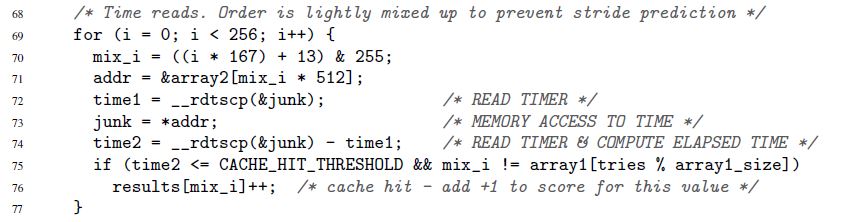
Here, in lines 72-74, the execution time of a single memory access operation is measured. True, Specter is not interested in nanoseconds. Time can be measured in "parrots". To parrots and seconds we will return.

Time-stamp counter

The key to fast and accurate time measurement is a special microprocessor counter. The value of this counter is usually stored in a separate register and is usually — but not always — accessible from user space. On different architectures, the counter is called differently:

1. time-stamp counter on x86
2. time base register on PowerPC
3. interval time counter on Itanium
4. etc.

Below, I will use the name “time-stamp counter” or TSC everywhere, although in reality I will mean any such counter, regardless of architecture.

Reading the value of a TSC is usually — but again not always — possible with a single instruction. Here is an example for x86. Strictly speaking, this is not a pure assembler instruction, but a GNU inline assembler:

uint32_t eax, edx; __asm__ __volatile__( "rdtsc" : "=a" (eax), "=d" (edx)); 

The "rdtsc" instruction places two 32-bit halves of the TSC register in the eax and edx registers. Of these, you can "glue" a single 64-bit value.

Once again, this (and similar) instructions in most cases can be called directly from user space. No system calls. Minimum overhead.

What needs to be done now to measure time?

1. Execute one such instruction at the beginning of the period of interest. Remember counter value
2. Execute one such instruction at the end. We believe that the value of the counter from the first instruction to the second will increase. Otherwise, why is it needed? Remember the second value
3. We consider the difference between the two saved values. This is our time.

It looks simple, but ...

The time measured by the described procedure is expressed in "parrots". It is not in seconds. But sometimes parrots are exactly what you need. There are situations when it is not the absolute values ​​of time intervals that are important, but how the various intervals correlate with each other. The above Specter example demonstrates exactly this situation. The duration of each individual memory access does not matter. It is only important that calls to one address will be executed much faster than to others (depending on whether the data is stored in the cache or main memory).

What if no parrots are needed, but seconds / microseconds / nanoseconds, etc.? There are two fundamentally different cases:

1. Nanoseconds are needed, but then. That is, it is permissible to make all the measurements in parrots first and save them somewhere for further processing (for example, in memory). And only after the measurements have been completed, slowly converting the collected parrots into seconds.
2. Nanoseconds are needed on the fly. For example, your measurement process has some kind of “consumer” that you do not control and who expects time in the “human” format

The first case is simple, the second one requires resourcefulness. Conversion should be as efficient as possible. If it consumes a lot of resources, it can greatly distort the measurement process. We'll talk about effective conversion below. Here we have identified this problem so far and turn to another.

Time-stamp counter-s are not as simple as we would like. On some architectures:

1. It is not guaranteed that the TSC is updated with high frequency. If a TSC is updated, say, once a microsecond, then it will not be possible to fix nanoseconds with its help
2. the frequency with which the TSC is updated may vary over time
3. on different CPUs present in the system, the TSC can be updated with different frequency
4. there may be a shift between TSC ticking on different CPUs.

Here is an example illustrating the last problem. Suppose we have a system with two CPUs: CPU1 and CPU2. Suppose that the TSC on the first CPU lags behind the second by the number of ticks, which is equivalent to 5 seconds. Suppose further that the system runs a thread that measures the computation time, which he himself does. To do this, the thread first reads the TSC value, then does the calculation, and then reads the second TSC value. If during all its life the thread remains on only one CPU - on any - then there are no problems. But what if the thread started on CPU1, measured the first TSC value there, and then in the middle of the calculations was moved by the operating system to CPU2, where it read the second TSC value? In this case, the calculations will seem 5 seconds longer than they actually are.

Due to the above problems, TSC cannot serve as a reliable source of time on some systems. However, on other systems “suffering” from the same problems, TSC can still be used. This is possible thanks to special architectural features:

1. hardware can generate a special interrupt each time the frequency at which the TSC is updated is changed. In this case, the equipment also provides the ability to find out the current frequency. Alternatively, the TSC update rate can be brought under the control of the operating system (see “Power ISA Version 2.06 Revision B, Book II, Chapter 5”)
2. hardware along with the TSC value can also provide the ID of the CPU on which this value is read (see Intel's RDTSCP instruction, "Intel 64 and IA-32 Architects Software Developer's Manual," Volume 2)
3. on some systems, you can programmatically adjust the TSC value for each CPU (see the Intel WRMSR instruction and the register IA32_TIME_STAMP_COUNTER, "Intel 64 and IA-32 Architectures Software Developer's Manual, Volume 3)

In general, the topic of how time counters are implemented on different architectures is fascinating and extensive. If you have time and interest, I recommend to dive. Among other things, you will find out, for example, that some systems allow you to programmatically find out if a TSC can serve as a reliable source of time.

So, there are many architectural implementations of TSC, each with its own characteristics. But it is interesting that a general trend has been established throughout this zoo. Modern hardware and operating systems strive to ensure that :

1. TSC ticks at the same frequency on every CPU in the system
2. this frequency does not change in time
3. between TSC ticking on different CPUs, there is no shift

When designing my library, I decided to proceed from this premise, and not from the vinaigrette of hardware implementations.

Library

I did not begin to lay on the hardware chips heaps of different architectures. Instead, I decided that my library would be focused on the modern trend. She has a purely empirical focus:

1. it allows you to experimentally test the reliability of TSC as a source of time
2. also allows you to experimentally calculate the parameters necessary for the rapid conversion of "ticks" in nanoseconds
3. in a natural way, the library provides convenient interfaces for reading TSC and converting ticks to nanoseconds on the fly

Library code is available here. It will be compiled and executed only on Linux.

In the code you can see the details of the implementation of all methods, which will be discussed further.

TSC reliability rating

The library provides an interface that returns two evaluations:

1. maximum offset between counters belonging to different CPUs. Only CPUs available to the process are considered. For example, if there are three CPUs available to the process, and at the same time TSC on these CPUs are 50, 150, 20, then the maximum shift will be 150-20 = 130. Naturally, experimentally, the library will not be able to get a real maximum shift, but it will give an estimate in which this shift will fit. What to do with the assessment next? How to use? This is already solved by client code. But the meaning is about the following. The maximum shift is the maximum value by which the measurement that the client code makes may be distorted. For example, in our example with three CPUs, the client code began to measure time on CPU3 (where TSC was 20), and finished on CPU2 (where TSC was 150). It turns out that in the measured interval, extra 130 ticks will creep in. And never again. The difference between CPU1 and CPU2 would be only 100 ticks. Having a rating of 130 ticks (in fact, it will be much more conservative), the client can decide whether he is satisfied with this magnitude of distortion or not.
2. Do TSC values ​​increase in series on the same or different CPUs? Here the idea is as follows. Suppose we have several CPUs. Suppose their watches are synchronized and ticking with the same frequency. Then, if you first measure the time on one CPU, and then measure it again — already on any of the available CPUs — then the second digit must be greater than the first.
   
   I will call this estimate below the TSC monotony estimate.
   

Now let's see how to get the first grade:

1. one of the available process CPU is declared "basic"
2. then all the other CPUs are sorted out, and for each of them a shift is calculated: TSC___CPU – TSC___CPU . This is done as follows:
   
   • a) take three successively (one after the other!) measured values: TSC_base_1, TSC_current, TSC_base_2 . Here, current indicates that the value was measured on the current CPU, and base on the base
   • b) TSC___CPU – TSC___CPU must lie in the interval [TSC_current – TSC_base_2, TSC_current – TSC_base_1] . This is on the assumption that TSC ticks with the same frequency on both CPUs.
   • c) steps a) -b) are repeated several times. Calculates the intersection of all intervals obtained in step b). The resulting interval is taken as the estimate of the shift TSC___CPU – TSC___CPU
   
   
3. After the estimated shift for each CPU relative to the base is obtained, it is easy to get an estimate of the maximum shift between all available CPUs:
   
   • a) calculate the minimum interval, which includes all the resulting intervals, obtained in step 2
   • b) the width of this interval is taken as an estimate of the maximum shift between TSC ticking on different CPUs.
   
   

To assess the monotony in the library, the following algorithm is implemented:

1. Suppose a process is available N CPU
2. Measure TSC on CPU1
3. Measure TSC on CPU2
4. ...
5. Measure TSC on CPUN
6. Measure TSC on CPU1 again
7. Check that the measured values ​​monotonously increase from the first to the last.

It is important here that the first and last values ​​are measured on the same CPU. And that's why. Suppose we have 3 CPUs. Suppose that the TSC on CPU2 is shifted by +100 ticks relative to the TSC on CPU1. Also assume that TSC on CPU3 is shifted by +100 ticks relative to TSC on CPU2. Consider the following chain of events:

• Read TSC on CPU1. Let the value 10 be obtained
• 2 ticks passed
• Read TSC on CPU2. Must be 112
• 2 ticks passed
• Read TSC on CPU3. Must be 214

So far, the clock looks synchronized. But let's again measure TSC on CPU1:

• 2 ticks passed
• Read TSC on CPU1. Must be 16

Oops! Monotony is broken. It turns out that measuring the first and last values ​​on the same CPU allows you to detect more or less large shifts between hours. The next question, of course: “How big is the shift?” The amount of shift that can be detected depends on the time that passes between successive TSC measurements. In the example above, this is just 2 ticks. Shifts between clocks greater than 2 ticks will be detected. Generally speaking, shifts that are less than the time that passes between successive measurements will not be detected. This means that the tighter the measurements in time are, the better. The accuracy of both estimates depends on this. The tighter the measurements are made:

• the lower the maximum shift estimate
• the more confidence in the monotony evaluation

In the next section we will talk about how to make dense measurements. Here I’ll add that while calculating the TSC reliability ratings, the library does many more simple checks for lice, for example:

• limited verification that TSC on different CPUs is ticking at the same speed
• check that the counters do change in time, and not just show the same value

Two methods for collecting meter values

In the library, I implemented two methods for collecting TSC values:

1. Switch between CPUs . In this method, all the data necessary for assessing the reliability of a TSC is collected by a single stream that “jumps” from one CPU to another. Both algorithms described in the previous section are suitable for this method and are not suitable for the other.
   There is no practical use for switching between CPUs. The method was implemented just for the sake of "play." The problem of the method is that the time required to drag the thread from one CPU to another is very long. Accordingly, a lot of time passes between successive measurements of TSC, and the accuracy of the estimates is very low. For example, a typical estimate for the maximum shift between TSC is obtained in the region of 23,000 ticks.
   
   Nevertheless, the method has a couple of advantages:
   
   • he is absolutely deterministic. If you need to consistently measure TSC on CPU1, CPU2, CPU3, then we just take and do it: switch to CPU1, read TSC, switch to CPU2, read TSC, and finally, switch to CPU3, read TSC
   • presumably, if the number of CPUs in the system grows very quickly, then the time to switch between them should grow much slower. Therefore, in theory, apparently, there can be a system - a very large system! - in which the use of the method will be justified. But nevertheless it is improbable
   
   
2. Measurements ordered by CAS . In this method, data is collected in parallel by multiple threads. On each available CPU, one thread is started. Measurements made by different threads are ordered in a single sequence using the “compare-and-swap” operation. Below is a piece of code that shows how this is done.
   The idea of ​​the method is borrowed from fio , a popular tool for generating I / O loads.
   
   The reliability estimates obtained with the power of this method already look very good. For example, the estimate of the maximum shift is obtained at the level of several hundred ticks. A monotony check allows you to catch the desynchronization of clocks within hundreds of ticks.
   
   However, the algorithms given in the previous section are not suitable for this method. For them, it is important that the TSC values ​​are measured in a predetermined order. The method of "measurements ordered by CAS" does not allow this. Instead, a long sequence of random measurements is first collected, and then the algorithms (already others) attempt to find in this sequence the values ​​read on the "suitable" CPUs.
   
   I will not give these algorithms here, so as not to abuse your attention. They can be seen in the code. There are many comments. Ideally, these algorithms are the same. A fundamentally new moment is a test of how statistically typed TSC sequences are statistically “qualitative”. It is also possible to set the minimum acceptable level of statistical significance for TSC reliability ratings.
   
   Theoretically, for VERY large systems, the method of “measurements ordered by CAS” can give poor results. The method requires that processors compete for access to a common memory cell. If there are a lot of processors, the match can be very tense. As a result, it will be difficult to create a measurement sequence with good statistical properties. However, at the moment such a situation seems unlikely.
   

I promised some code. Here is how building the measurements in a single chain with the help of CAS.

  for ( uint64_t i = 0; i < arg->probes_count; i++ ) { uint64_t seq_num = 0; uint64_t tsc_val = 0; do { __atomic_load( seq_counter, &seq_num, __ATOMIC_ACQUIRE); __sync_synchronize(); tsc_val = WTMLIB_GET_TSC(); } while ( !__atomic_compare_exchange_n( seq_counter, &seq_num, seq_num + 1, false, __ATOMIC_ACQ_REL, __ATOMIC_RELAXED)); arg->tsc_probes[i].seq_num = seq_num; arg->tsc_probes[i].tsc_val = tsc_val; } 

This code is executed on every available CPU. All threads have access to the shared variable seq_counter . Before reading the TSC, the stream reads the value of this variable and stores it in the variable seq_num . Then reads TSC. Then it tries to atomically increase seq_counter by one, but only if the value of the variable has not changed since it was read. If the operation is successful, it means that the thread managed to “stake out” the sequence number stored in seq_num after the measured TSC value. The next sequence number that can be staked out (perhaps already in another thread) will be one more. For this number is taken from the variable seq_counter , and each successful call __atomic_compare_exchange_n() increases this variable by one.


Another point worth mentioning here is the concern that all measurement flows start more or less at the same time. We are interested in the fact that the TSC values ​​read on different CPUs are mixed together as best as possible. We are not satisfied with the situation when, for example, one thread will start first, finish its work, and only then all the others will start. The resulting TSC sequence will have useless properties. From it will not work to extract any estimates. The simultaneous start of all threads is important - and for this the library has taken action.

Tick ​​conversion to nanoseconds on the fly

After checking the reliability of TSC, the second big library assignment is to convert ticks to nanoseconds on the fly. The idea of ​​this conversion, I borrowed from the already mentioned fio. However, I had to make several significant improvements, because, as shown by my analysis, in fio itself, the conversion procedure does not work well enough. It turns out low accuracy.

Immediately begin with an example.

Ideally, I would like to convert tics to nanoseconds like this:
ns_time = tsc_ticks / tsc_per_ns
We want the time spent on conversion to be minimal. Therefore, we aim to use only integer arithmetic. Let's see what it may threaten us.

If tsc_per_ns = 3 , then simple integer division, from the point of view of accuracy, works fine: ns_time = tsc_ticks / 3 .

But what if tsc_per_ns = 3.333 ? If this number is rounded to 3, the conversion accuracy will be very low. :
ns_time = (tsc_ticks * factor) / (3.333 * factor) .

factor , . - . , . – . , x86 10+ . , .

:
ns_time = (tsc_ticks * factor / 3.333) / factor .

– . (factor / 3.333) . – - . , factor . – .

factor ? , factor . , , , 64- . , «» . , .

, factor . , . TSC : 3.333 * 1000000000 * 60 * 60 * 24 * 365 = 105109488000000000 . 64- : 18446744073709551615 / 105109488000000000 ~ 175.5 . , (factor / 3.333) , . : factor <= 175.5 * 3.333 ~ 584.9 . , , 512. , :

ns_time = (tsc_ticks * 512 / 3.333) / 512

:

ns_time = tsc_ticks * 153 / 512

. , . 1000000000 * 60 * 60 * 24 * 365 = 31536000000000000 . : 105109488000000000 * 153 / 512 = 31409671218750000 . 126328781250000 , 126328781250000 / 1000000000 / 60 / 60 ~ 35 .

. . ? . . :

ns_time = tsc_ticks * 1258417 / 4194304 (1)

119305 1 ( 0.2 ). . , , . ? ?

:

tsc_ticks = (tsc_ticks_per_1_hour * number_of_hours) + tsc_ticks_remainder

tsc_ticks_per_1_hour , number_of_hours tsc_ticks . , , . tsc_ticks , . , tsc_ticks_remainder . , , . , , (1).

Is done. . .

, . 1 . :

tsc_ticks = modulus * number_of_moduli_periods + tsc_ticks_remainder

, :

ns_per_remainder = (tsc_ticks_remainder * factor / tsc_per_nsec) / factor

( , tsc_ticks_remainder < modulus ):

modulus * (factor / tsc_per_nsec) <= UINT64_MAX
factor <= (UINT64_MAX / modulus) * tsc_per_nsec
2 ^ shift <= (UINT64_MAX / modulus) * tsc_per_nsec


, , . . , , , .

, shift , :

factor = 2 ^ shift
mult = factor / tsc_per_nsec


:

ns_per_remainder = (tsc_ticks_remainder * mult) >> shift


, . , – tsc_ticks_remainder number_of_moduli_periods tsc_ticks . , . , . modulus :

modulus = 2 ^ remainder_bit_length

Then:

number_of_moduli_periods = tsc_ticks >> remainder_bit_length
tsc_ticks_remainder = tsc_ticks & (modulus - 1)

Fine. , tsc_ticks number_of_moduli_periods tsc_ticks_remainder . , tsc_ticks_remainder . , , modulus . :

ns_per_moduli = ns_per_modulus * number_of_moduli_periods

ns_per_modulus . , . , , modulus . modulus , , , modulus .

ns_per_modulus = (modulus * mult) >> shift

Everything! , « ». :

1. tsc_ticks
2. number_of_moduli_periods = tsc_ticks >> remainder_bit_length
3. tsc_ticks_remainder = tsc_ticks & (modulus - 1)
4. ns = ns_per_modulus * number_of_moduli_periods + (tsc_ticks_remainder * mult) >> shift

remainder_bit_length , modulus, ns_per_modulus , mult shift .

, . , performance- .

So here. , :)

, mult ? :

mult = factor / tsc_per_nsec

: tsc_per_nsec ?
– . tsc_per_nsec (tsc_per_sec / 1000000000) . Those.:

mult = factor * 1000000000 / tsc_per_sec

:

1. tsc_per_sec , tsc_per_msec , ?
2. tsc_per_sec ?

. fio . . , , tsc_per_msec = 2599998 . tsc_per_sec = 2599998971 . , : 0.999999626. , , 374 . – tsc_per_sec .

… tsc_per_sec ?

:

start_sytem_time = clock_gettime()
start_tsc = WTMLIB_GET_TSC()
-
end_system_time = clock_gettime()
end_tsc = WTMLIB_GET_TSC()


«- » — . , . , . , end_system_time start_system_time 0,6 . tsc_per_sec = (end_tsc – start_tsc) / 0,6 .

tsc_per_sec . «» - tsc_per_sec , .

, , clock_gettime() WTMLIB_GET_TSC() . , WTMLIB_GET_TSC() , clock_gettime() . TSC. tsc_per_sec . tsc_per_sec . .

Conclusion

, .

. . :

• – –
• modulus ( )?
• , modulus , , ( tsc_per_msec tsc_per_sec ). ?
• TSC . ?
• . , fio timespec. :
  
  tp->tv_sec = nsecs / 1000000000ULL;
  
  , TSC . , ,
  

. , .

, fio, , 700-900 ( ). - . fio. , . , .

!