Face Detection Video: Raspberry Pi and Neural Compute Stick

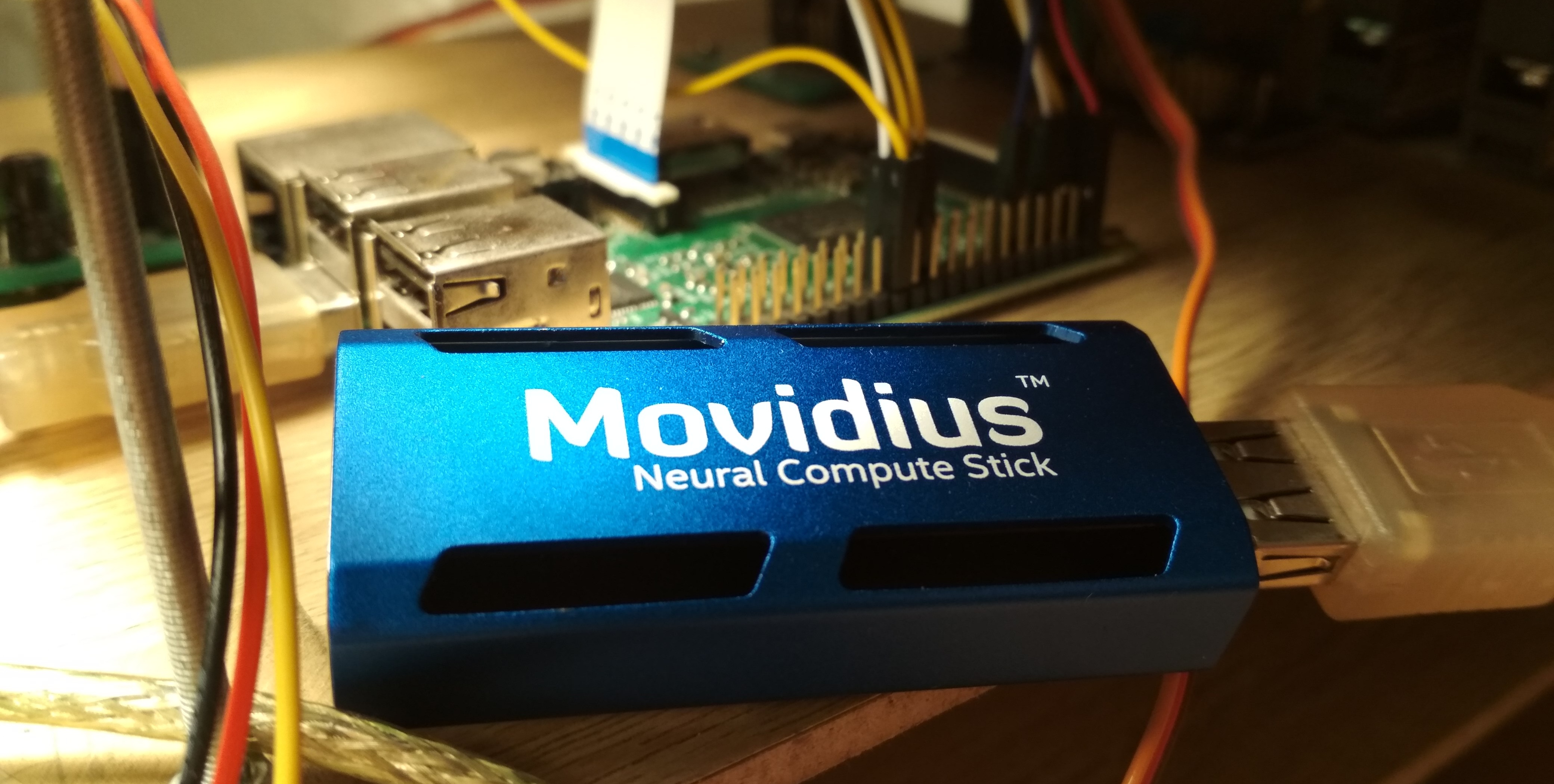
About a year ago, Intel Movidius released a device for the effective inference of convolutional neural networks - the Movidius Neural Compute Stick (NCS). This device allows the use of neural networks for recognition or detection of objects in conditions of limited power consumption, including robotics tasks. NCS has a USB interface and consumes no more than 1 watt. In this article I will talk about the experience of using NCS with the Raspberry Pi for the task of detecting faces in video, including both the training of the Mobilenet-SSD detector and its launch on the Raspberry.

All code can be found in my two repositories: detector training and face detection demo .



In my first article I already wrote about face detection using NCS: then it was a YOLOv2 detector, which I converted from Darknet format to Caffe format, and then launched on NCS. The conversion process turned out to be nontrivial: since these two formats set the last detector layer differently, the neural network output had to be parsed separately on the CPU, using a piece of code from Darknet. In addition, this detector did not satisfy me both in speed (up to 5.1 FPS on my laptop) and in accuracy - I later became convinced that because of the sensitivity to image quality from it, it is difficult to get a good result on the Raspberry Pi.
')
In the end, I decided to just train my detector. The choice fell on the SSD detector with the Mobilenet encoder: the lightweight Mobilenet convolutions make it possible to achieve high speed without much loss in quality, while the SSD detector itself is not inferior to YOLO and works on NCS out of the box.

Detector training

Architecture

The code for learning detector is located here .

I decided to use the ready Mobilenet-SSD detector trained in PASCAL VOC0712 and add it to face detection. Firstly, it helps to train the net faster, and secondly, you don’t have to reinvent the wheel.

The original project included a gen.py script that literally collected the model's .prototxt file, substituting the input parameters. I transferred it to my project, expanding the functionality a bit. This script allows you to generate four types of configuration files:

• train : at the entrance there is an LMDB training base, at the exit there is a layer with calculation of the loss function and its gradients, there is a BatchNorm
• test : at the entrance - test LMDB base, at the exit - a layer with a quality calculation (mean average precision), there is a BatchNorm
• deploy : input - image, output - layer with predictions, BatchNorm is absent
• deploy_bn : at the entrance - an image, at the exit - a layer with predictions, there is a BatchNorm

I added the last option later so that the scripts could load and convert the grid from BatchNorm without touching the LMDB database - otherwise, if there was no database, nothing worked. (Actually, it seems to me strange that in Caffe a data source is set in the network architecture - this is at least not very practical).


I slightly corrected the network architecture. List of changes:

• Obviously, the number of classes changed to 1 (not counting the background).
• The restrictions on the aspect ratio of the cut patches during training: have changed since $$$[0.5,2.0]$on $$$[0.7,1.4]$(I decided to simplify the task a little and not study on too stretched pictures).
• Of the default frames, only square boxes remain, two for each cell. I have greatly reduced their size, since the faces are significantly smaller than the objects in the classical problem of detecting objects.

Caffe calculates the size of the default framework as follows: having a minimum frame size $$$s$and maximum $$$L$it creates a small and large frame with dimensions $$$s$and $$$\ sqrt {sL}$. Since I wanted to detect as small faces as possible, I calculated the full stride for each layer of detections and equated the minimum frame size to it. With such parameters, the small default framework will be located close to each other and will not intersect. So at least we have a guarantee that the intersection with the object will exist for some frame. I set the maximum size twice. For layers conv16_2, conv17_2 I put the dimensions on the eye, the same. In this way, $$$s, L$for all layers were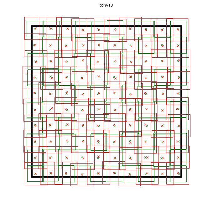: $$$(16.32), (32.64), (64.128), (128.214), (214,300), (214,300)$

Data

I used two datasets : WIDER Face and FDDB . WIDER contains a lot of pictures with very small and blurred faces, and FDDB more to large images of faces (and an order of magnitude less than WIDER). The annotation format is slightly different, but these are details.

I didn’t use all the data for training: I threw out too small faces (less than six pixels or less than 2% of the image width), threw out all the images with the aspect ratio less than 0.5 or more than 2, threw out all the images marked as “blurred” in WIDER dataset, since they corresponded for the most part to very small individuals, and I had to at least somehow align the ratio of small and large individuals. After that, I made all the frames square, expanding the smallest side: I decided that I was not very interested in the proportions of the face, and the task for the neural network was a little simpler. I also threw out all the black and white pictures, which were few and on which the database build script falls.

To use them for training and testing, you need to build an LMDB base from them. How it's done:

• For each image, markup is created in the .xml format.
• A train.txt file is train.txt with lines like "path/to/image.png path/to/labels.xml" , the same is created for test.
• A test_name_size.txt file is test_name_size.txt with strings of the form "test_image_name height width"
• A labelmap.prototxt file is labelmap.prototxt with numeric matching labels.

The ssd-caffe/scripts/create_annoset.py (an example from the Makefile):

 python3 /opt/movidius/ssd-caffe/scripts/create_annoset.py --anno-type=detection \ --label-map-file=$(wider_dir)/labelmap.prototxt --min-dim=0 --max-dim=0 \ --resize-width=0 --resize-height=0 --check-label --encode-type=jpg --encoded \ --redo $(wider_dir) \ $(wider_dir)/trainval.txt $(wider_dir)/WIDER_train/lmdb/wider_train_lmdb ./data 

Using two datasets at the same time means only that you need to carefully merge the corresponding files in pairs, not forgetting to correctly register the paths, and also to mix the file for training.

After that, you can start learning.

Training

The code for learning the model can be found in my Colab Notebook .

I did the training at Google Collaboration, because my laptop was barely able to test the mesh, and I was stuck in training. Colaboratory allowed me to train the grid fairly quickly and for free. The trick is that I had to write an SSD-Caffe compilation script for Collaboration (which includes such strange things as recompiling boost and editing sources), which takes about 40 minutes. More details can be found in my previous publication .

Colaboratory has one more feature: after 12 hours, the car dies, permanently erasing all the data. The best way to avoid data loss is to install a Google disk into the system and save network weights into it every 500-1000 learning iterations.

As for my detector, in one session at Colaboratory he managed to unlearn 4500 iterations, and he fully studied in two sessions.

The quality of predictions (average average precision) on the test data set that I selected (merged by WIDER and FDDB with the limitations listed above) was about 0.87 for the best model. To measure the mAP on the scales saved during the training, there is a script scripts/plot_map.py .

Detector operation on (very strange) example from dataset:

Run on NCS

The face detection demo is here .

To compile a neural network for the Neural Compute Stick, you need Movidius NCSDK : it contains utilities for compiling and profiling neural networks, as well as C ++ and Python API. It is worth noting that a second version was recently released that was not compatible with the first one: all API functions were renamed for some reason, the internal format of neural networks was changed, FIFOs were added to interact with NCS and (finally) automatic conversion from float 32 bit to float 16 bit, which is so lacking in C ++. I updated all my projects to the second version, but left a couple of crutches for compatibility with the first one.

After learning the detector, it is worthwhile to merge the BatchNorm layers with the next convolutions to speed up the neural network. This is handled by the merge_bn.py script from here , which I also borrowed from the Mobilenet-SSD project.

Then you need to call the mvNCCompile utility, for example:

 mvNCCompile -s 12 -o graph_ssd -w ssd-face.caffemodel ssd-face.prototxt 

In the project's Makefile there is a graph_ssd target for this. The resulting graph_ssd file is a description of the neural network in a format understood by NCS.

Now about how to interact with the device itself. The process is not very complicated, but requires a fairly large amount of code. The sequence of actions is approximately as follows:

• Get device descriptor by ordinal number
• Open device
• Read the compiled file of the neural network in the buffer (as a binary file)
• Create an empty calculation graph for NCS
• Place the graph on the device, using the data from the file, and select for it a FIFO on input / output; file buffer can now be freed
• Run detector:
  
  • Get the image from the camera (or from any other source)
  • Process it: scale to the desired size, convert to float32 and result in a range [-1,1]
  • Download the image to the device and request the inference
  • Request a result (the program will be blocked until the result is received)
  • Parse the result, select the object frames (about the format - below)
  • Display image with predictions
  
  
• Free all resources: delete the FIFO and the calculation graph, close the device and delete its descriptor

Almost for every action with NCS there is a separate function, and in C ++ it looks very cumbersome, and you have to carefully monitor the release of all resources. In order not to load the code, I created a wrapper class for working with NCS . In it, all the initialization work is hidden in the constructor and the load_file function, and in the release of resources, in the destructor, and working with NCS comes down to calling 2-3 class methods. In addition, there is a convenient function to explain the errors that have occurred.

Create a wrapper by passing the input size and output size (number of elements) to the constructor:

 NCSWrapper NCS(NETWORK_INPUT_SIZE*NETWORK_INPUT_SIZE*3, NETWORK_OUTPUT_SIZE); 

We load the compiled file with a neural network, simultaneously initializing everything we need:

 if (!NCS.load_file("./models/face/graph_ssd")) { NCS.print_error_code(); return 0; } 

Let's convert the image to float32 ( image is cv::Mat in CV_32FC3 format) and upload it to the device:

 if(!NCS.load_tensor_nowait((float*)image.data)) { NCS.print_error_code(); break; } 

We get the result ( result - this is a free float pointer, the result buffer is supported by a wrapper); until the end of the calculations, the program is blocked:

 if(!NCS.get_result(result)) { NCS.print_error_code(); break; } 

In fact, there is a method in the wrapper that allows you to load data and get the result simultaneously: load_tensor((float*)image.data, result) . I refused to use it for a reason: using separate methods, you can slightly speed up the execution of the code. After the image is loaded, the CPU will remain idle until the result of executing with NCS (in this case it is about 100 ms) comes, and at this time you can do some useful work: read the new frame and convert it, and display the previous detections. . This is how the demo program is implemented, in my case it slightly increases the FPS. You can go ahead and start image processing and face detection asynchronously in two different threads - it really works and allows you to speed up a bit more, but it is not implemented in the demo program.

The detector returns a float array of size 7*(keep_top_k+1) as a result. Here, keep_top_k is the parameter specified in the .prototxt file of the model and indicating how many detections (in order of decreasing confidence) must be returned. This parameter, as well as the parameter responsible for filtering detections by the minimum confidence value, and the parameters of non maximum suppression can be configured in the model’s .prototxt file in the most recent layer. It should be noted that if Caffe returns as many detections as it was found in the image, then NCS always returns keep_top_k detections so that the size of the array is constant.

The result array itself is organized as follows: if we treat it as a matrix with keep_top_k+1 rows and 7 columns, then in the first row, in the first element there will be the number of detections, and starting with the second row, the detections themselves will be in the format "garbage, class_index, class_probability, x_min, y_min, x_max, y_max" . The coordinates are in the range [0,1], so they will need to be multiplied by the height / width of the image. In the remaining elements of the array will be garbage. In this case, the maximum maximum suppression is performed automatically, even before the result is obtained (it seems, right on the NCS).

Startup features on the Raspberry Pi

The demo program itself can be run either on a regular computer or a laptop with Ubuntu, or on Raspberry Pi with Raspbian Stretch. I use the Raspberry Pi 2 model B, but the demo should work on other models. The project's makefile contains two targets for mode switching: make switch_desk for a computer / laptop and make switch_rpi for a Raspberry Pi. The principal difference in the program code is only that in the first case, OpenCV is used to read data from the camera, and in the second case, the RaspiCam library. To run the demo on Raspberry you need to compile and install it.

Now a very important point: installing NCSDK. If you follow the standard installation instructions on the Raspberry Pi, it won't end well: the installer will try to pull in and compile SSD-Caffe and Tensorflow. Instead, NCSDK must be compiled in API-only mode . In this mode, only C ++ and Python API will be available (that is, it will not be possible to compile and profile neural network graphs). This means that the graph of the neural network must first be compiled on a regular computer and then copied to Raspberry. For convenience, I added two compiled files to the repository, for YOLO and for SSD.

Another interesting point is the purely physical connection of the NCS to the Raspberry. It would seem easy to connect it to a USB-connector, but you need to remember that its body will block the other three connectors (it is quite healthy, since it performs the function of a radiator). The easiest way out is to connect it via a USB cable.

It is also worth bearing in mind that the execution speed will differ for different USB versions (for this particular network: 102 ms for USB 3.0, 92 ms for USB 2.0).

Now about the power of the NCS. According to the documentation, it consumes up to 1 watt (with 5 volts on the USB connector it will be up to 200 ma; for comparison: the Raspberry camera consumes up to 250 ma). When powered from a conventional 5 volt charger, 2 amps all work fine. However, when you try to connect two or more NCS to the Raspberry, problems may arise. In this case, it is recommended to use a USB splitter with external power supply.

On Raspberry, the demo runs slower than on a computer / laptop: 7.2 FPS vs. 10.4 FPS. This is due to several factors: first, it is impossible to get rid of computing on the CPU, and they are performed much slower; secondly, the speed of data transmission affects (for USB 2.0).

Also, for comparison, I tried to run a face detector from my first article on Raspberry YOLOv2, but it worked very badly: at a speed of 3.6 FPS, it misses a lot of faces even on simple frames. Apparently, it is very sensitive to the parameters of the input image, the quality of which in the case of the Raspberry camera is far from ideal. The SSD is much more stable, although I had to tweak the video parameters a bit in the RapiCam settings. he, too, sometimes misses faces in the frame, but he does this quite rarely. To increase stability in real applications, you can add a simple centroid tracker .

By the way: the same can be reproduced in Python, there is a tutorial on PyImageSearch (used by Mobilenet-SSD for the object detection task).

Other ideas

I also tested a couple of ideas for accelerating the neural network itself:

The first idea: you can leave only the detection of the layers conv11 and conv13 , and remove all the extra layers. The result is a detector that detects only small faces and works a little faster. Overall, not worth it.

The second idea was interesting, but it did not work: I tried to discard convolutions with weights close to zero from the neural network, hoping that it would become faster. However, such bundles turned out to be few, and their removal only slightly slowed down the neural network (the only guess is that this is due to the fact that the number of channels ceased to be a power of two).

Conclusion

I’ve been thinking about finding faces on Raspberry for quite some time, as a subtask of my robotic project. I did not like the classic detectors in terms of speed and quality, and I decided to try neural network methods, at the same time testing the Neural Compute Stick, as a result of which two projects appeared on GitHub and three articles on Habré (including the current one). In general, the result suits me - most likely, I will use this detector in my robot (perhaps there will be another article about it). It is worth noting that my decision may not be optimal - nevertheless, this is an educational project, made partly out of curiosity towards NCS. Nevertheless, I hope that this article will be useful to someone.