Enron Corporation is one of the most famous figures in the American business of the 2000s. This was facilitated not by their sphere of activity (electricity and contracts for its supply), but by the response due to fraud in it. For 15 years, corporate earnings grew rapidly, and work in it promised good wages. But it ended just as quickly: in the period 2000-2001. the share price fell from $ 90 / piece to almost zero due to the discovery of declared income fraud. Since then, the word "Enron" has become a household name and acts as a label for companies that operate in a similar way.

During the trial, 18 people (including the biggest defendants in this case: Andrew Fastov, Jeff Skilling and Kenneth Lay) were convicted.

However, an archive of electronic correspondence between employees of the company, better known as Enron Email Dataset, and insider information about the income of employees of this company were published.

The article will consider the sources of these data and build a model based on them, which allows to determine whether a person is suspected of fraud. Sounds interesting? Then, welcome under habrakat.

Dataset description

Enron dataset (dataset) is a consolidated set of open data that contains records of people working in a memorable corporation with a corresponding name.

It can be divided into 3 parts:

• payments_features - a group characterizing financial movements;
• stock_features - group, reflecting the attributes associated with the shares;
• email_features is a group that reflects information about the email of a particular person in an aggregated form.

Of course, there is also a target variable that indicates whether the person is suspected of fraud (the 'poi' sign ).

Let's load our data and start with working with them:

import pickle with open("final_project/enron_dataset.pkl", "rb") as data_file: data_dict = pickle.load(data_file) 

Then turn the data_dict set into the Pandas dataframe for more convenient work with the data:

 import pandas as pd import warnings warnings.filterwarnings('ignore') source_df = pd.DataFrame.from_dict(data_dict, orient = 'index') source_df.drop('TOTAL',inplace=True) 

Group the signs in accordance with the previously specified types. This should facilitate the work with the data afterwards:

 payments_features = ['salary', 'bonus', 'long_term_incentive', 'deferred_income', 'deferral_payments', 'loan_advances', 'other', 'expenses', 'director_fees', 'total_payments'] stock_features = ['exercised_stock_options', 'restricted_stock', 'restricted_stock_deferred','total_stock_value'] email_features = ['to_messages', 'from_poi_to_this_person', 'from_messages', 'from_this_person_to_poi', 'shared_receipt_with_poi'] target_field = 'poi' 

Financial data

In this data there is a well-known NaN, and it expresses a familiar gap in the data. In other words, the author of the dataset could not find any information on a particular attribute related to a specific line in the data frame. As a consequence, we can assume that NaN is 0, since there is no information about a specific trait.

 payments = source_df[payments_features] payments = payments.replace('NaN', 0) 

Data checking

When comparing with the original PDF underlying the dataset, it turned out that the data is slightly distorted, since the total_payments field is not for all the lines in the data frame of payments . You can check this as follows:

 errors = payments[payments[payments_features[:-1]].sum(axis='columns') != payments['total_payments']] errors.head()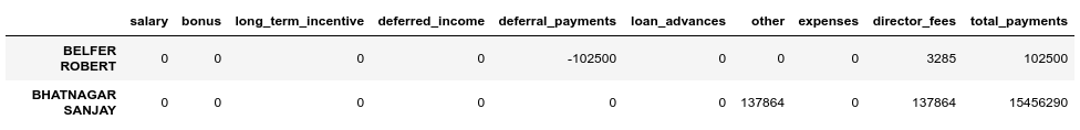 

We see that BELFER ROBERT and BHATNAGAR SANJAY have incorrect payment amounts.

This error can be corrected by shifting the data in the erroneous lines to the left or right and counting the sum of all payments again:

 import numpy as np shifted_values = payments.loc['BELFER ROBERT', payments_features[1:]].values expected_payments = shifted_values.sum() shifted_values = np.append(shifted_values, expected_payments) payments.loc['BELFER ROBERT', payments_features] = shifted_values shifted_values = payments.loc['BHATNAGAR SANJAY', payments_features[:-1]].values payments.loc['BHATNAGAR SANJAY', payments_features] = np.insert(shifted_values, 0, 0) 

Share data

 stocks = source_df[stock_features] stocks = stocks.replace('NaN', 0) 

Perform a validation check in this case as well:

 errors = stocks[stocks[stock_features[:-1]].sum(axis='columns') != stocks['total_stock_value']] errors.head()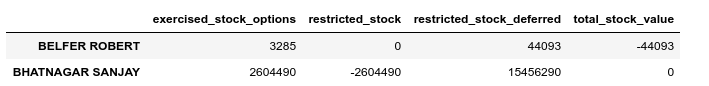 

Correct the same error in promotions:

 shifted_values = stocks.loc['BELFER ROBERT', stock_features[1:]].values expected_payments = shifted_values.sum() shifted_values = np.append(shifted_values, expected_payments) stocks.loc['BELFER ROBERT', stock_features] = shifted_values shifted_values = stocks.loc['BHATNAGAR SANJAY', stock_features[:-1]].values stocks.loc['BHATNAGAR SANJAY', stock_features] = np.insert(shifted_values, 0, shifted_values[-1]) 

Email Summary

If NaN was equivalent to 0 for these finances or shares, and this fit into the final result for each of these groups, in the case of email, NaN is more reasonable to replace with some default value. To do this, you can use the Imputer:

 from sklearn.impute import SimpleImputer imp = SimpleImputer() 

However, we will consider the default value for each category (if a person is suspected of fraud) separately:

 target = source_df[target_field] email_data = source_df[email_features] email_data = pd.concat([email_data, target], axis=1) email_data_poi = email_data[email_data[target_field]][email_features] email_data_nonpoi = email_data[email_data[target_field] == False][email_features] email_data_poi[email_features] = imp.fit_transform(email_data_poi) email_data_nonpoi[email_features] = imp.fit_transform(email_data_nonpoi) email_data = email_data_poi.append(email_data_nonpoi) 

Final dataset after correction:

 df = payments.join(stocks) df = df.join(email_data) df = df.astype(float) 

Emissions

At the final step of this stage, we’ll remove all outliers that can distort the training. At the same time, there is always the question: how much data can we remove from the sample and not lose as a learning model? I followed the advice of one of the lecturers leading the course on ML (machine learning) at Udacity - “Remove 10 pieces and check for emissions again”.

 first_quartile = df.quantile(q=0.25) third_quartile = df.quantile(q=0.75) IQR = third_quartile - first_quartile outliers = df[(df > (third_quartile + 1.5 * IQR)) | (df < (first_quartile - 1.5 * IQR))].count(axis=1) outliers.sort_values(axis=0, ascending=False, inplace=True) outliers = outliers.head(10) outliers 

At the same time, we will not delete records that are outliers and are suspected of fraud. The reason is that there are only 18 lines with such data, and we cannot sacrifice them, as this may lead to a lack of examples for learning. As a result, we remove only those who are not suspected of fraud, but at the same time have a large number of signs, according to which emissions are observed:

 target_for_outliers = target.loc[outliers.index] outliers = pd.concat([outliers, target_for_outliers], axis=1) non_poi_outliers = outliers[np.logical_not(outliers.poi)] df.drop(non_poi_outliers.index, inplace=True) 

Reduction to the final form

Normalize our data:

 from sklearn.preprocessing import scale df[df.columns] = scale(df) 

Let's bring the target variable target to a compatible view:

 target.drop(non_poi_outliers.index, inplace=True) target = target.map({True: 1, False: 0}) target.value_counts()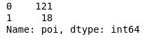 

As a result, 18 suspects and 121 those who did not fall under suspicion.

Feature selection

Perhaps one of the most key points before learning any model is the selection of the most important features.

Multicollinearity test

 import matplotlib.pyplot as plt import seaborn as sns %matplotlib inline sns.set(style="whitegrid") corr = df.corr() * 100 # Select upper triangle of correlation matrix mask = np.zeros_like(corr, dtype=np.bool) mask[np.triu_indices_from(mask)] = True # Set up the matplotlib figure f, ax = plt.subplots(figsize=(15, 11)) # Generate a custom diverging colormap cmap = sns.diverging_palette(220, 10) # Draw the heatmap with the mask and correct aspect ratio sns.heatmap(corr, mask=mask, cmap=cmap, center=0, linewidths=1, cbar_kws={"shrink": .7}, annot=True, fmt=".2f")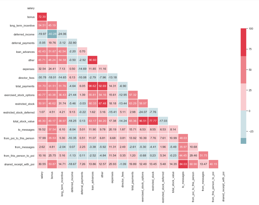 

As can be seen from the image, we have a pronounced relationship between 'loan_advanced' and 'total_payments', as well as between 'total_stock_value' and 'restricted_stock'. As mentioned earlier, 'total_payments' and 'total_stock_value' are just the result of adding all the indicators in a particular group. Therefore, they can be removed:

 df.drop(columns=['total_payments', 'total_stock_value'], inplace=True) 

Creating new features

There is also an assumption that suspects wrote to accomplices more often than employees who were not involved in this. And as a result, the share of such messages should be greater than the share of messages to ordinary employees. Based on this statement, you can create new signs reflecting the percentage of incoming / outgoing related to the suspects:

 df['ratio_of_poi_mail'] = df['from_poi_to_this_person']/df['to_messages'] df['ratio_of_mail_to_poi'] = df['from_this_person_to_poi']/df['from_messages'] 

Eliminating unnecessary signs

In the toolkit of people associated with ML, there are many excellent tools for selecting the most significant attributes (SelectKBest, SelectPercentile, VarianceThreshold, etc.). In this case, RFECV will be used because it includes cross-validation, which allows you to calculate the most important features and check them on all subsets of the sample:

 from sklearn.model_selection import train_test_split X_train, X_test, y_train, y_test = train_test_split(df, target, test_size=0.2, random_state=42) 

 from sklearn.feature_selection import RFECV from sklearn.ensemble import RandomForestClassifier forest = RandomForestClassifier(random_state=42) rfecv = RFECV(estimator=forest, cv=5, scoring='accuracy') rfecv = rfecv.fit(X_train, y_train) plt.figure() plt.xlabel("Number of features selected") plt.ylabel("Cross validation score of number of selected features") plt.plot(range(1, len(rfecv.grid_scores_) + 1), rfecv.grid_scores_, '--o') indices = rfecv.get_support() columns = X_train.columns[indices] print('The most important columns are {}'.format(','.join(columns)))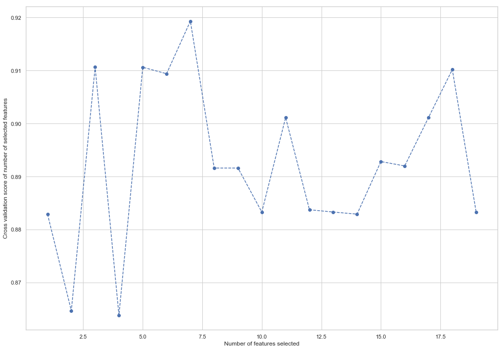 

As you can see, RandomForestClassifier considered that only 7 signs out of 18 are important. Using the rest leads to a decrease in the accuracy of the model.

 The most important columns are bonus, deferred_income, other, exercised_stock_options, shared_receipt_with_poi, ratio_of_poi_mail, ratio_of_mail_to_poi 

These 7 features will be used further in order to simplify the model and reduce the risk of retraining:

• bonus
• deferred_income
• other
• exercised_stock_options
• shared_receipt_with_poi
• ratio_of_poi_mail
• ratio_of_mail_to_poi

Let's change the structure of the training and test samples for the future training of the model:

 X_train = X_train[columns] X_test = X_test[columns] 

This is the end of the first part, describing the use of Enron Dataset as an example of a classification task in ML. Based on materials from the course Introduction to Machine Learning at Udacity. There is also a python notebook , reflecting the entire sequence of actions.

The second part is here