Learning and testing neural networks on PyTorch using Ignite

Hi, Habr, in this article I will talk about the ignite library, with which you can easily train and test neural networks using the PyTorch framework.

With ignite, you can write cycles for learning the network literally in a few lines, add standard metrics from the box, save the model, etc. Well, for those who moved from TF to PyTorch, we can say that the ignite library is Keras for PyTorch.

The article will detail the example of training a neural network for a classification task using ignite

Add more fire to PyTorch

I will not waste time talking about how cool the PyTorch framework is. The one who has already used it, understands what I am writing about. But, with all its merits, it is still low-level in terms of writing cycles for learning, testing, testing neural networks.

If we look at the official examples of using the PyTorch framework, we will see in the training code of the grid at least two cycles of iterations per epoch and training sample batch:

for epoch in range(1, epochs + 1): for batch_idx, (data, target) in enumerate(train_loader): # ... 

The main idea of ​​the ignite library is to factor these cycles into a single class, while allowing the user to interact with these cycles using event handlers.

As a result, in the case of standard deep learning tasks, we can pretty well save on the number of lines of code. Less lines - less mistakes!

For example, for comparison, on the left is the code for learning and validating the model using ignite , and on the right - on pure PyTorch: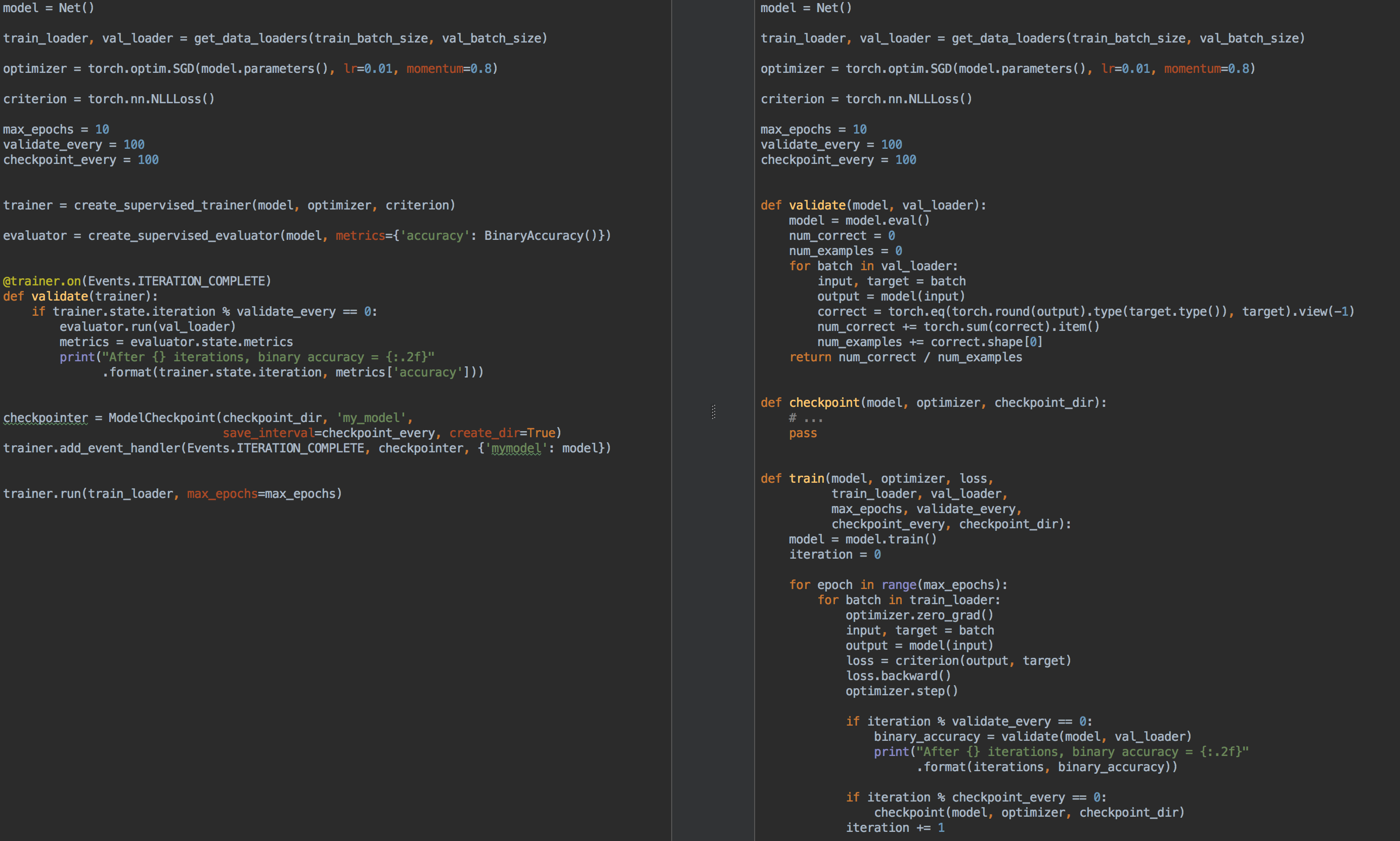

So again, what good is ignite ?

• for each task, there is no need to write for epoch in range(n_epochs) and for batch in data_loader cycles for epoch in range(n_epochs) each task.
• allows for better factorization of the code
• allows you to calculate base metrics out of the box
• provides “buns” of type
  
  • saving the latest and best models (also the optimizer and learning rate scheduler) during training,
  • early learning stop
  • etc
• integrates easily with visualization tools: tensorboardX, visdom, ...

In a sense, as already mentioned, the ignite library can be compared to all known Keras and its API for learning and testing networks. Also, the ignite library at first glance is very similar to the tnt library, since initially both libraries pursued the same goals and have similar ideas for their implementation.

So, we light:

 pip install pytorch-ignite 

or

 conda install ignite -c pytorch 

Further on a concrete example we will look at the API library ignite .

Classification task with ignite

In this part of the article, we will consider a school example of learning a neural network for a classification task using the ignite library.

So, let's take a simple dataset with pictures of fruit with kaggle . The task is to compare each class with fruit to the corresponding class.

Before using ignite , let's define the main components:

Data flow (dataflow):

• trainer batch bootloader, train_loader
• check sample fetch batch loader, val_loader

Model:

• take a small squeezeNet grid from torchvision

Optimization Algorithm:

• take SGD

Loss function:

• Cross-entropy

 from pathlib import Path import numpy as np import torch from torch.utils.data import Dataset, DataLoader from torch.utils.data.dataset import Subset from torchvision.datasets import ImageFolder from torchvision.transforms import Compose, RandomResizedCrop, RandomVerticalFlip, RandomHorizontalFlip from torchvision.transforms import ColorJitter, ToTensor, Normalize FRUIT360_PATH = Path(".").resolve().parent / "input" / "fruits-360_dataset" / "fruits-360" device = "cuda" train_transform = Compose([ RandomHorizontalFlip(), RandomResizedCrop(size=32), ColorJitter(brightness=0.12), ToTensor(), Normalize(mean=[0.5, 0.5, 0.5], std=[0.5, 0.5, 0.5]) ]) val_transform = Compose([ RandomResizedCrop(size=32), ToTensor(), Normalize(mean=[0.5, 0.5, 0.5], std=[0.5, 0.5, 0.5]) ]) batch_size = 128 num_workers = 8 train_dataset = ImageFolder((FRUIT360_PATH /"Training").as_posix(), transform=train_transform, target_transform=None) val_dataset = ImageFolder((FRUIT360_PATH /"Test").as_posix(), transform=val_transform, target_transform=None) train_loader = DataLoader(train_dataset, batch_size=batch_size, shuffle=True, num_workers=num_workers, drop_last=True, pin_memory="cuda" in device) val_loader = DataLoader(val_dataset, batch_size=batch_size, shuffle=True, num_workers=num_workers, drop_last=False, pin_memory="cuda" in device) 

 import torch.nn as nn from torchvision.models.squeezenet import squeezenet1_1 model = squeezenet1_1(pretrained=False, num_classes=81) model.classifier[-1] = nn.AdaptiveAvgPool2d(1) model = model.to(device) 

 import torch.nn as nn from torch.optim import SGD optimizer = SGD(model.parameters(), lr=0.01, momentum=0.5) criterion = nn.CrossEntropyLoss() 

So now it's time to start ignite :

 from ignite.engine import Engine, _prepare_batch def process_function(engine, batch): model.train() optimizer.zero_grad() x, y = _prepare_batch(batch, device=device) y_pred = model(x) loss = criterion(y_pred, y) loss.backward() optimizer.step() return loss.item() trainer = Engine(process_function) 

Let's see what this code means.

Engine Engine

The class ignite.engine.Engine is the framework of the library, and the object of this class is trainer :

 trainer = Engine(process_function) 

It is defined with the process_function input function for processing a single batch and serves to implement passes through the training set. Inside the ignite.engine.Engine class, the following happens:

 while epoch < max_epochs: # run once on data for batch in data: output = process_function(batch) 

Let's return to the process_function function:

 def process_function(engine, batch): model.train() optimizer.zero_grad() x, y = _prepare_batch(batch, device=device) y_pred = model(x) loss = criterion(y_pred, y) loss.backward() optimizer.step() return loss.item() 

We see that inside the function we, as usual in the case of learning the model, calculate the predictions y_pred , calculate the loss function loss and gradients. The latter allow updating model weights: optimizer.step() .

In general, there are no restrictions on the process_function function code. We only note that it takes two arguments as input: an Engine object ( trainer in our case) and a batch from the data loader. Therefore, for example, to test a neural network, we can define another object of the ignite.engine.Engine class, in which the input function simply calculates the predictions, and implement a pass through the test sample one single time. Read about it below.

So, the above code only defines the necessary objects without running the training. In principle, in the minimal example, you can call the method:

 trainer.run(train_loader, max_epochs=10) 

and this code is enough to "quietly" (without any output of intermediate results) train the model.

 from ignite.engine import create_supervised_trainer trainer = create_supervised_trainer(model, optimizer, criterion, device) 

Of course, in practice, the above example is of little interest, so let's add the following options for the “trainer”:

• display of the loss function value every 50 iterations
• running the calculation of metrics on the training set with a fixed model
• running the calculation of metrics on the test sample after each epoch
• saving model parameters after each epoch
• keeping the top three models
• change in learning rate depending on the era (learning rate scheduling)
• early-stopping

Events and Event Handlers

To add the above options for the trainer, the ignite library provides an event system and the launch of custom event handlers. Thus, the user can control an Engine class object at each stage:

• engine started / completed launch
• era began / ended
• batch iteration started / ended

and run your code on every event.

Display of loss function values

To do this, simply define the function in which the output will be displayed on the screen, and add it to the "trainer":

 from ignite.engine import Events log_interval = 50 @trainer.on(Events.ITERATION_COMPLETED) def log_training_loss(engine): iteration = (engine.state.iteration - 1) % len(train_loader) + 1 if iteration % log_interval == 0: print("Epoch[{}] Iteration[{}/{}] Loss: {:.4f}" .format(engine.state.epoch, iteration, len(train_loader), engine.state.output)) 

Actually there are two ways to add an event handler: via add_event_handler , or through the on decorator. The same as above can be done like this:

 from ignite.engine import Events log_interval = 50 def log_training_loss(engine): # ... trainer.add_event_handler(Events.ITERATION_COMPLETED, log_training_loss) 

Note that any arguments can be passed to the event handling function. In general, this function will look like this:

 def custom_handler(engine, *args, **kwargs): pass trainer.add_event_handler(Events.ITERATION_COMPLETED, custom_handler, *args, **kwargs) #  @trainer.on(Events.ITERATION_COMPLETED, *args, **kwargs) def custom_handler(engine, *args, **kwargs): pass 

So, let's start training on one epoch and see what happens:

 output = trainer.run(train_loader, max_epochs=1) 

 Epoch[1] Iteration[50/322] Loss: 4.3459 Epoch[1] Iteration[100/322] Loss: 4.2801 Epoch[1] Iteration[150/322] Loss: 4.2294 Epoch[1] Iteration[200/322] Loss: 4.1467 Epoch[1] Iteration[250/322] Loss: 3.8607 Epoch[1] Iteration[300/322] Loss: 3.6688 

Not bad! Come on.

Running the calculation of metrics on the training and test samples

Let's calculate the following metrics: average accuracy, average completeness after each epoch on the part of the training and the entire test sample. Note that we will calculate the metrics on the part of the training sample after each training epoch, and not during the training. Thus, the measurement of efficiency will be more accurate, since the model does not change during the calculation.

So, we define the metrics:

 from ignite.metrics import Loss, CategoricalAccuracy, Precision, Recall metrics = { 'avg_loss': Loss(criterion), 'avg_accuracy': CategoricalAccuracy(), 'avg_precision': Precision(average=True), 'avg_recall': Recall(average=True) } 

Next, we will create two engines for evaluating the model using ignite.engine.create_supervised_evaluator :

 from ignite.engine import create_supervised_evaluator # ,  device = “cuda”    train_evaluator = create_supervised_evaluator(model, metrics=metrics, device=device) val_evaluator = create_supervised_evaluator(model, metrics=metrics, device=device) 

We create two engines so that we can attach additional event handlers to one of them ( val_evaluator ) to save the model and stop learning early (more on this later).

Let's also take a closer look at how the engine for model evaluation is defined, namely, how the process_function input function is defined for processing a single batch:

 def create_supervised_evaluator(model, metrics={}, device=None): if device: model.to(device) def _inference(engine, batch): model.eval() with torch.no_grad(): x, y = _prepare_batch(batch, device=device) y_pred = model(x) return y_pred, y engine = Engine(_inference) for name, metric in metrics.items(): metric.attach(engine, name) return engine 

We continue further. Let us randomly select a part of the training sample on which we will calculate the metrics:

 import numpy as np from torch.utils.data.dataset import Subset indices = np.arange(len(train_dataset)) random_indices = np.random.permutation(indices)[:len(val_dataset)] train_subset = Subset(train_dataset, indices=random_indices) train_eval_loader = DataLoader(train_subset, batch_size=batch_size, shuffle=True, num_workers=num_workers, drop_last=True, pin_memory="cuda" in device) 

Next, let's determine at what point in the training we will start the calculation of metrics and will produce output to the screen:

 @trainer.on(Events.EPOCH_COMPLETED) def compute_and_display_offline_train_metrics(engine): epoch = engine.state.epoch print("Compute train metrics...") metrics = train_evaluator.run(train_eval_loader).metrics print("Training Results - Epoch: {} Average Loss: {:.4f} | Accuracy: {:.4f} | Precision: {:.4f} | Recall: {:.4f}" .format(engine.state.epoch, metrics['avg_loss'], metrics['avg_accuracy'], metrics['avg_precision'], metrics['avg_recall'])) @trainer.on(Events.EPOCH_COMPLETED) def compute_and_display_val_metrics(engine): epoch = engine.state.epoch print("Compute validation metrics...") metrics = val_evaluator.run(val_loader).metrics print("Validation Results - Epoch: {} Average Loss: {:.4f} | Accuracy: {:.4f} | Precision: {:.4f} | Recall: {:.4f}" .format(engine.state.epoch, metrics['avg_loss'], metrics['avg_accuracy'], metrics['avg_precision'], metrics['avg_recall'])) 

You can run!

 output = trainer.run(train_loader, max_epochs=1) 

We get on the screen

 Epoch[1] Iteration[50/322] Loss: 3.5112 Epoch[1] Iteration[100/322] Loss: 2.9840 Epoch[1] Iteration[150/322] Loss: 2.8807 Epoch[1] Iteration[200/322] Loss: 2.9285 Epoch[1] Iteration[250/322] Loss: 2.5026 Epoch[1] Iteration[300/322] Loss: 2.1944 Compute train metrics... Training Results - Epoch: 1 Average Loss: 2.1018 | Accuracy: 0.3699 | Precision: 0.3981 | Recall: 0.3686 Compute validation metrics... Validation Results - Epoch: 1 Average Loss: 2.0519 | Accuracy: 0.3850 | Precision: 0.3578 | Recall: 0.3845 

Already better!

Few details
Let's take a little look at the previous code. The reader may have noticed the following line of code:

 metrics = train_evaluator.run(train_eval_loader).metrics 

and, probably, there was a question about the type of the object obtained from the function train_evaluator.run(train_eval_loader) , which has the metrics attribute.

In fact, the Engine class has a structure called state (of type State ) in order to be able to pass data between event handlers. This state attribute contains basic information about the current epoch, iteration, number of epochs, etc. It can also be used to transfer any user data, including the results of calculating metrics.

 state = train_evaluator.run(train_eval_loader) metrics = state.metrics #   train_evaluator.run(train_eval_loader) metrics = train_evaluator.state.metrics 

Calculation of metrics during training

If the task is a huge learning sample and the calculation of metrics after each training epoch is expensive, and yet I would like to see some metrics change during training, then the following RunningAverage event handler can be used out of the box. For example, we want to calculate and display the accuracy of the classifier:

 acc_metric = RunningAverage(CategoryAccuracy(...), alpha=0.98) acc_metric.attach(trainer, 'running_avg_accuracy') @trainer.on(Events.ITERATION_COMPLETED) def log_running_avg_metrics(engine): print("running avg accuracy:", engine.state.metrics['running_avg_accuracy']) 

To use the RunningAverage functionality, you need to install ignite from sources:

 pip install git+https://github.com/pytorch/ignite 

Change learning speed (scheduling)

There are several ways to change the speed of learning with ignite . Next, we consider the simplest method by calling the lr_scheduler.step() function at the beginning of each epoch.

 from torch.optim.lr_scheduler import ExponentialLR lr_scheduler = ExponentialLR(optimizer, gamma=0.8) @trainer.on(Events.EPOCH_STARTED) def update_lr_scheduler(engine): lr_scheduler.step() #    : if len(optimizer.param_groups) == 1: lr = float(optimizer.param_groups[0]['lr']) print("Learning rate: {}".format(lr)) else: for i, param_group in enumerate(optimizer.param_groups): lr = float(param_group['lr']) print("Learning rate (group {}): {}".format(i, lr)) 

Saving the best models and other parameters during training

During training, it would be great to record the weights of the best model on the disk, as well as periodically save the model weights, optimizer parameters, and learning speed change parameters. The latter can be useful in order to resume learning from the last saved state.

Ignite has a special ModelCheckpoint class for this. So let's create a ModelCheckpoint event ModelCheckpoint and store the best model by the precision value on the test set. In this case, we define the score_function function, which score_function the value of accuracy in the event handler and it decides whether to save the model or not:

 from ignite.handlers import ModelCheckpoint def score_function(engine): val_avg_accuracy = engine.state.metrics['avg_accuracy'] return val_avg_accuracy best_model_saver = ModelCheckpoint("best_models", filename_prefix="model", score_name="val_accuracy", score_function=score_function, n_saved=3, save_as_state_dict=True, create_dir=True) # "best_models" -    1     #   -> {filename_prefix}_{name}_{step_number}_{score_name}={abs(score_function_result)}.pth # save_as_state_dict=True, #   `state_dict` val_evaluator.add_event_handler(Events.COMPLETED, best_model_saver, {"best_model": model}) 

Now we will create another ModelCheckpoint event ModelCheckpoint in order to save the learning state every 1000 iterations:

 training_saver = ModelCheckpoint("checkpoint", filename_prefix="checkpoint", save_interval=1000, n_saved=1, save_as_state_dict=True, create_dir=True) to_save = {"model": model, "optimizer": optimizer, "lr_scheduler": lr_scheduler} trainer.add_event_handler(Events.ITERATION_COMPLETED, training_saver, to_save) 

So, almost everything is ready, add the last element:

Early-stopping

Let's add another event handler that will stop learning if there is no improvement in the quality of the model over 10 epochs. The quality of the model will again be evaluated using the score_function score_function .

 from ignite.handlers import EarlyStopping early_stopping = EarlyStopping(patience=10, score_function=score_function, trainer=trainer) val_evaluator.add_event_handler(Events.EPOCH_COMPLETED, early_stopping) 

Start learning

In order to run the training we just need to call the run() method. We will train the model for 10 epochs:

 max_epochs = 10 output = trainer.run(train_loader, max_epochs=max_epochs) 

 Learning rate: 0.01 Epoch[1] Iteration[50/322] Loss: 2.7984 Epoch[1] Iteration[100/322] Loss: 1.9736 Epoch[1] Iteration[150/322] Loss: 4.3419 Epoch[1] Iteration[200/322] Loss: 2.0261 Epoch[1] Iteration[250/322] Loss: 2.1724 Epoch[1] Iteration[300/322] Loss: 2.1599 Compute train metrics... Training Results - Epoch: 1 Average Loss: 1.5363 | Accuracy: 0.5177 | Precision: 0.5477 | Recall: 0.5178 Compute validation metrics... Validation Results - Epoch: 1 Average Loss: 1.5116 | Accuracy: 0.5139 | Precision: 0.5400 | Recall: 0.5140 Learning rate: 0.008 Epoch[2] Iteration[50/322] Loss: 1.4076 Epoch[2] Iteration[100/322] Loss: 1.4892 Epoch[2] Iteration[150/322] Loss: 1.2485 Epoch[2] Iteration[200/322] Loss: 1.6511 Epoch[2] Iteration[250/322] Loss: 3.3376 Epoch[2] Iteration[300/322] Loss: 1.3299 Compute train metrics... Training Results - Epoch: 2 Average Loss: 3.2686 | Accuracy: 0.1977 | Precision: 0.1792 | Recall: 0.1942 Compute validation metrics... Validation Results - Epoch: 2 Average Loss: 3.2772 | Accuracy: 0.1962 | Precision: 0.1628 | Recall: 0.1918 Learning rate: 0.006400000000000001 Epoch[3] Iteration[50/322] Loss: 0.9016 Epoch[3] Iteration[100/322] Loss: 1.2006 Epoch[3] Iteration[150/322] Loss: 0.8892 Epoch[3] Iteration[200/322] Loss: 0.8141 Epoch[3] Iteration[250/322] Loss: 1.4005 Epoch[3] Iteration[300/322] Loss: 0.8888 Compute train metrics... Training Results - Epoch: 3 Average Loss: 0.7368 | Accuracy: 0.7554 | Precision: 0.7818 | Recall: 0.7554 Compute validation metrics... Validation Results - Epoch: 3 Average Loss: 0.7177 | Accuracy: 0.7623 | Precision: 0.7863 | Recall: 0.7611 Learning rate: 0.005120000000000001 Epoch[4] Iteration[50/322] Loss: 0.8490 Epoch[4] Iteration[100/322] Loss: 0.8493 Epoch[4] Iteration[150/322] Loss: 0.8100 Epoch[4] Iteration[200/322] Loss: 0.9165 Epoch[4] Iteration[250/322] Loss: 0.9370 Epoch[4] Iteration[300/322] Loss: 0.6548 Compute train metrics... Training Results - Epoch: 4 Average Loss: 0.7047 | Accuracy: 0.7713 | Precision: 0.8040 | Recall: 0.7728 Compute validation metrics... Validation Results - Epoch: 4 Average Loss: 0.6737 | Accuracy: 0.7778 | Precision: 0.7955 | Recall: 0.7806 Learning rate: 0.004096000000000001 Epoch[5] Iteration[50/322] Loss: 0.6965 Epoch[5] Iteration[100/322] Loss: 0.6196 Epoch[5] Iteration[150/322] Loss: 0.6194 Epoch[5] Iteration[200/322] Loss: 0.3986 Epoch[5] Iteration[250/322] Loss: 0.6032 Epoch[5] Iteration[300/322] Loss: 0.7152 Compute train metrics... Training Results - Epoch: 5 Average Loss: 0.5049 | Accuracy: 0.8282 | Precision: 0.8393 | Recall: 0.8314 Compute validation metrics... Validation Results - Epoch: 5 Average Loss: 0.5084 | Accuracy: 0.8304 | Precision: 0.8386 | Recall: 0.8328 Learning rate: 0.0032768000000000007 Epoch[6] Iteration[50/322] Loss: 0.4433 Epoch[6] Iteration[100/322] Loss: 0.4764 Epoch[6] Iteration[150/322] Loss: 0.5578 Epoch[6] Iteration[200/322] Loss: 0.3684 Epoch[6] Iteration[250/322] Loss: 0.4847 Epoch[6] Iteration[300/322] Loss: 0.3811 Compute train metrics... Training Results - Epoch: 6 Average Loss: 0.4383 | Accuracy: 0.8474 | Precision: 0.8618 | Recall: 0.8495 Compute validation metrics... Validation Results - Epoch: 6 Average Loss: 0.4419 | Accuracy: 0.8446 | Precision: 0.8532 | Recall: 0.8442 Learning rate: 0.002621440000000001 Epoch[7] Iteration[50/322] Loss: 0.4447 Epoch[7] Iteration[100/322] Loss: 0.4602 Epoch[7] Iteration[150/322] Loss: 0.5345 Epoch[7] Iteration[200/322] Loss: 0.3973 Epoch[7] Iteration[250/322] Loss: 0.5023 Epoch[7] Iteration[300/322] Loss: 0.5303 Compute train metrics... Training Results - Epoch: 7 Average Loss: 0.4305 | Accuracy: 0.8579 | Precision: 0.8691 | Recall: 0.8596 Compute validation metrics... Validation Results - Epoch: 7 Average Loss: 0.4262 | Accuracy: 0.8590 | Precision: 0.8685 | Recall: 0.8606 Learning rate: 0.002097152000000001 Epoch[8] Iteration[50/322] Loss: 0.4867 Epoch[8] Iteration[100/322] Loss: 0.3090 Epoch[8] Iteration[150/322] Loss: 0.3721 Epoch[8] Iteration[200/322] Loss: 0.4559 Epoch[8] Iteration[250/322] Loss: 0.3958 Epoch[8] Iteration[300/322] Loss: 0.4222 Compute train metrics... Training Results - Epoch: 8 Average Loss: 0.3432 | Accuracy: 0.8818 | Precision: 0.8895 | Recall: 0.8817 Compute validation metrics... Validation Results - Epoch: 8 Average Loss: 0.3644 | Accuracy: 0.8713 | Precision: 0.8784 | Recall: 0.8707 Learning rate: 0.001677721600000001 Epoch[9] Iteration[50/322] Loss: 0.3557 Epoch[9] Iteration[100/322] Loss: 0.3692 Epoch[9] Iteration[150/322] Loss: 0.3510 Epoch[9] Iteration[200/322] Loss: 0.3446 Epoch[9] Iteration[250/322] Loss: 0.3966 Epoch[9] Iteration[300/322] Loss: 0.3451 Compute train metrics... Training Results - Epoch: 9 Average Loss: 0.3315 | Accuracy: 0.8954 | Precision: 0.9001 | Recall: 0.8982 Compute validation metrics... Validation Results - Epoch: 9 Average Loss: 0.3559 | Accuracy: 0.8818 | Precision: 0.8876 | Recall: 0.8847 Learning rate: 0.0013421772800000006 Epoch[10] Iteration[50/322] Loss: 0.3340 Epoch[10] Iteration[100/322] Loss: 0.3370 Epoch[10] Iteration[150/322] Loss: 0.3694 Epoch[10] Iteration[200/322] Loss: 0.3409 Epoch[10] Iteration[250/322] Loss: 0.4420 Epoch[10] Iteration[300/322] Loss: 0.2770 Compute train metrics... Training Results - Epoch: 10 Average Loss: 0.3246 | Accuracy: 0.8921 | Precision: 0.8988 | Recall: 0.8925 Compute validation metrics... Validation Results - Epoch: 10 Average Loss: 0.3536 | Accuracy: 0.8731 | Precision: 0.8785 | Recall: 0.8722 

Now check the models and parameters saved to disk:

 ls best_models/ model_best_model_10_val_accuracy=0.8730994.pth model_best_model_8_val_accuracy=0.8712978.pth model_best_model_9_val_accuracy=0.8818188.pth 

and

 ls checkpoint/ checkpoint_lr_scheduler_3000.pth checkpoint_optimizer_3000.pth checkpoint_model_3000.pth 

Predictions by a trained model

To begin with, we will create a test data loader (for example, let's take a validation sample) so that the data batch consists of images and their indices:

 class TestDataset(Dataset): def __init__(self, ds): self.ds = ds def __len__(self): return len(self.ds) def __getitem__(self, index): return self.ds[index][0], index test_dataset = TestDataset(val_dataset) test_loader = DataLoader(test_dataset, batch_size=batch_size, shuffle=False, num_workers=num_workers, drop_last=False, pin_memory="cuda" in device) 

Using ignite, we will create a new prediction engine for test data. To do this, we define the inference_update function, which gives the result of the prediction and the image index. To improve accuracy, we will also use the well-known “test time augmentation” (TTA) trick.

 import torch.nn.functional as F from ignite._utils import convert_tensor def _prepare_batch(batch): x, index = batch x = convert_tensor(x, device=device) return x, index def inference_update(engine, batch): x, indices = _prepare_batch(batch) y_pred = model(x) y_pred = F.softmax(y_pred, dim=1) return {"y_pred": convert_tensor(y_pred, device='cpu'), "indices": indices} model.eval() inferencer = Engine(inference_update) 

Next, create event handlers that will notify about the prediction stage and save the predictions to the selected array:

 @inferencer.on(Events.EPOCH_COMPLETED) def log_tta(engine): print("TTA {} / {}".format(engine.state.epoch, n_tta)) n_tta = 3 num_classes = 81 n_samples = len(val_dataset) #     y_probas_tta = np.zeros((n_samples, num_classes, n_tta), dtype=np.float32) @inferencer.on(Events.ITERATION_COMPLETED) def save_results(engine): output = engine.state.output tta_index = engine.state.epoch - 1 start_index = ((engine.state.iteration - 1) % len(test_loader)) * batch_size end_index = min(start_index + batch_size, n_samples) batch_y_probas = output['y_pred'].detach().numpy() y_probas_tta[start_index:end_index, :, tta_index] = batch_y_probas 

Before starting the process, let's load the best model:

 model = squeezenet1_1(pretrained=False, num_classes=64) model.classifier[-1] = nn.AdaptiveAvgPool2d(1) model = model.to(device) model_state_dict = torch.load("best_models/model_best_model_10_val_accuracy=0.8730994.pth") model.load_state_dict(model_state_dict) 

Run:

 inferencer.run(test_loader, max_epochs=n_tta) > TTA 1 / 3 > TTA 2 / 3 > TTA 3 / 3 

Next, in a standard way, we take the average of the predictions of TTA and calculate the index of the class with the highest probability:

 y_probas = np.mean(y_probas_tta, axis=-1) y_preds = np.argmax(y_probas, axis=-1) 

And now we can calculate once again the accuracy of the model according to the obtained predictions:

 from sklearn.metrics import accuracy_score y_test_true = [y for _, y in val_dataset] accuracy_score(y_test_true, y_preds) > 0.9310369676443035 

, , . , , , ignite .

ignite

.

github

• fast neural transfer
• reinforcement learning
• dcgan

Conclusion

, ignite Facebook (. ). 0.1.0, API (Engine, State, Events, Metric, ...) . , , , pull request- github .

Thanks for attention!