Outputting the curve function for smoothly limiting parameters, signals and not only in Wolfram Mathematica
There are a number of tasks in which the range of output values should be limited, while the input data cannot guarantee this. In addition to forced situations, signal limiting can also be a purposeful task - for example, when compressing a signal or implementing an “overdrive” effect.
The simplest implementation of the constraint is to force it to a certain value when a certain level is exceeded. For example, for a sinusoid with increasing amplitude, it will look like this:

')
The role of the limiter here is the Clip function, whose argument is the input signal and the parameters of the limit, and the result of the function is the output signal.
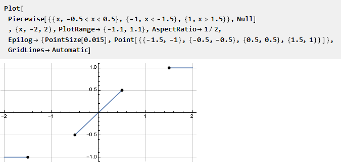
Let's look at the graph of the Clip function separately:
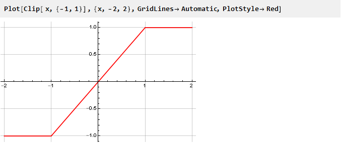
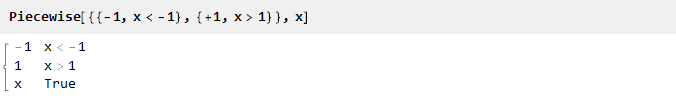
It shows that while we do not exceed the limits, the output value is equal to the input value and the signal does not change; if the output value is exceeded, the output value does not depend in any way and remains at the same level. In fact, we have a piecewise continuous function made up of three others: y = -1, y = x and y = 1, selected depending on the argument, and equivalent to the following record:
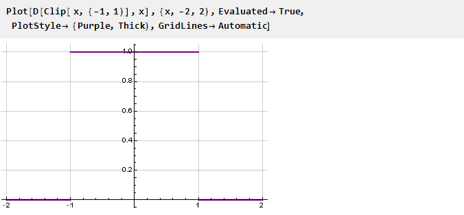
The transition between functions is quite dramatic; and looks tempting to make it smoother. Mathematically, this sharpness is due to the fact that the derivatives of the functions at the junction points do not coincide. This is easy to see by plotting the derivative of the Clip function:
Thus, to ensure the smoothness of the constraint function, it is necessary to ensure the equality of the derivatives at the docking points. And since the extreme functions of our constants, the derivatives of which are equal to zero, then the derivatives of the constraint function at the junction points must also be zero. Next, we will consider several such functions that provide smooth docking.
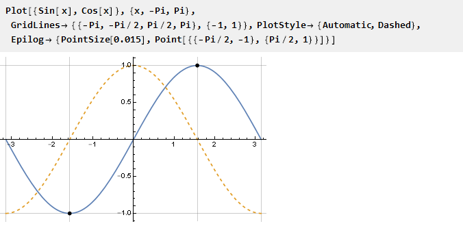
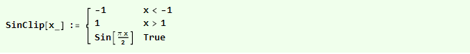
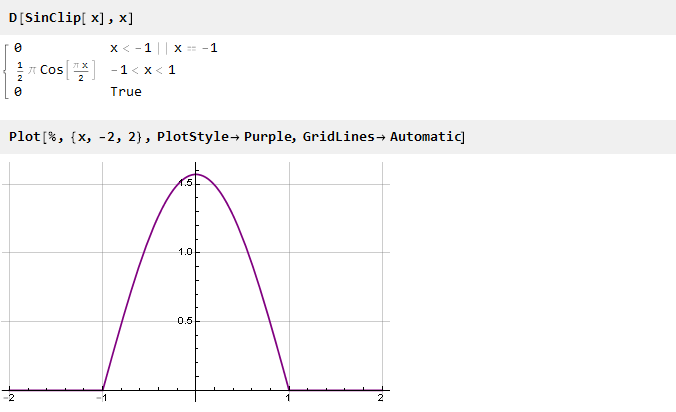
The simplest thing is to use the sin function on the interval from -pi / 2 to pi / 2, at the boundaries of which the values of the derivative are zero by definition:
It is only necessary to scale the arguments so that the unit is projected onto Pi / 2. Now we can define the actual limiting function:
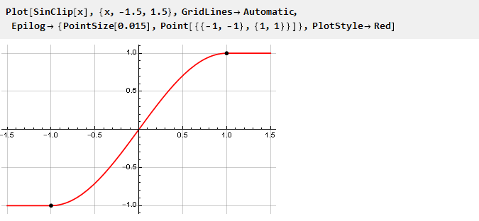
And build its schedule:
Since the limits of the limitation are strictly defined here, the limitation is defined by scaling the input signal followed by (if necessary) reverse scaling.
There is also no situation in which the input signal is transmitted to the output without distortion - the lower the gain level, the lower the level of distortion due to the limitation - but the signal is distorted anyway.
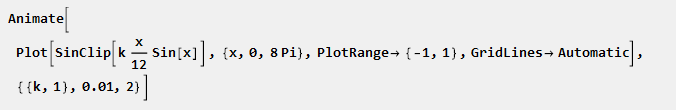
The effect of the gain parameter on signal distortion can be seen in dynamics:
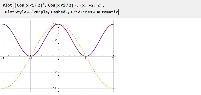
Let's look at the derivative of our function:
It already has no discontinuities in the values, but there are discontinuities in the derivative (the second, if we take it from the original function). In order to eliminate it, you can go the opposite way - first form a smooth derivative, and then integrate it to obtain the desired function.
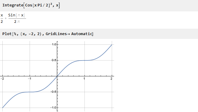
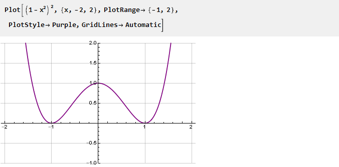
The easiest way to zero the derived points -1 and 1 is to simply square the function - all negative values of the function will become positive and, accordingly, there will be excesses at the intersection points of the function with zero.
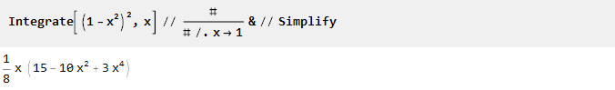
Find the primitive:
It now remains to scale it along the ordinate axis. For this we find its value at point 1:
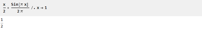
And we divide it into it (yes, it is here that this elementary multiplication by 2, but not always the case):
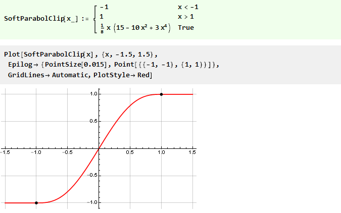
Thus, the final restriction function will take the form:
Using trigonometric functions in some cases can be somewhat wasteful. Therefore, we will try to build the function we need, while remaining within the framework of elementary mathematical operations.
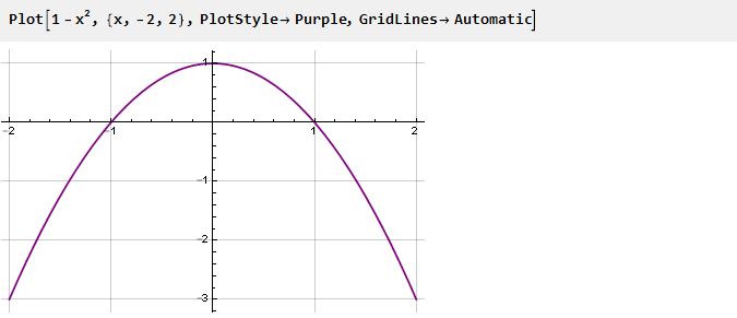
Consider a parabola:
Since it already has an inflection point at zero, we can use the same part on the interval {0,1} for docking with constants. For negative values, you need to move it down and to the left:

and for positive ones - to reflect vertically and horizontally:

And our function with a parabola will look like:
Let's return to our parabola, turn it over and move it up one unit:
This will be a derivative of our function. To make it smoother at the docking points, squared, thus nullifying the second derivative:
We integrate and scale:
We get an even smoother function:
Here we will try to achieve smoothness at the docking points for even higher derivatives. To do this, first define the function as a polynomial with unknown coefficients, and try to find the coefficients themselves by solving a system of equations.
Let's start with the 1st derivative:
2nd:
3rd:
All these coefficients look as if they have some kind of logic. We write down the factors, multiplying them by the value of the degree at x; and in order not to write the same thing every time, we automate the process of finding coefficients:
It looks like the binomial coefficients. We make a bold assumption that this is what they are, and based on this, we write the generalized formula:

Check:
It looks like the truth [1] . It remains only to calculate the scale factor to bring the edges to unity:
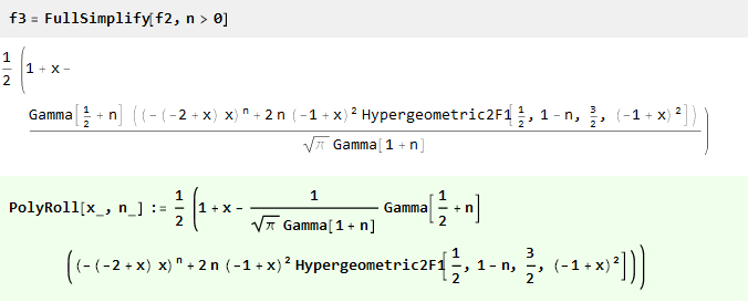
And after scaling and simplifying, we find that our knowledge of mathematics is somewhat outdated [2] :
Thus, we have obtained a generating function of order n, in which the n-1 first derivatives will be equal to zero:
Let's see what happened:
And since our generalized formula turned out to be continuous, if you wish, you can use non-integer parameter values:
You can also build graphs of derivatives reduced to the same scale:
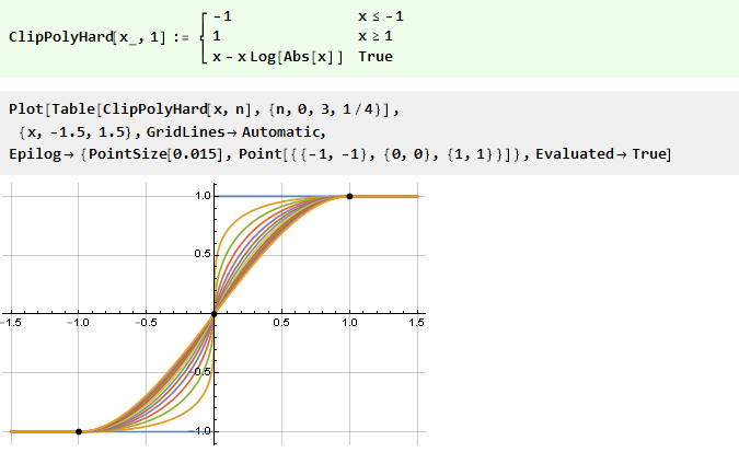
It would be tempting to be able to adjust the degree of "stiffness" of the constraint.
Let us return to our inverted parabola and add the coefficient at degree x:

The greater the n, the more our derivative is “square”, and its primitive is, respectively, sharp:
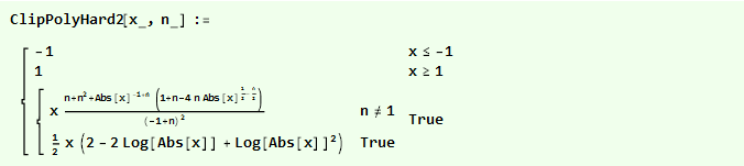
We calculate the antiderivative and adjust the scale:
Now let's try to set the fractional step for the parameter:
As we see, in the negative part, not for all n there is a correct solution, but in the right (positive) part, the conditions we need are still met — so for negative values we can simply use it in an inverted form with a reversed argument. And since the domain of definition of the parameter is no longer limited to positive integers, it is possible to simplify the formula by replacing 2n with n:

And replacing n with n-1, you can make the formula a little more beautiful:
Since when n is equal to unity, we get the division by zero, we will try to find the limit:
The limit is found, which means that now you can define [3] a function for n equal to 1 and consider it for all n large zero:
If we initially square our inverted parabola, we get an even smoother function:
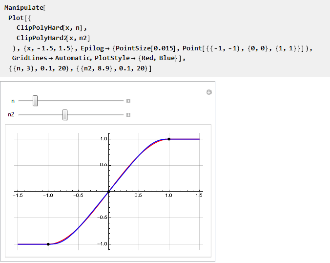
And we can compare them on one chart:
Let's look at the following function:
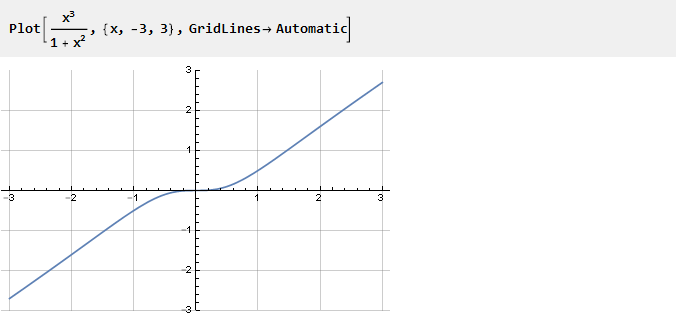
It appeared not by chance.
If you remove the unit from it, x 2 will be reduced and just x will remain, that is, the inclined line. Thus, the smaller the value of x, the greater the influence of the unit in the denominator, creating the curvature we need. And considering this function at different scales, one can control the degree of this curvature:

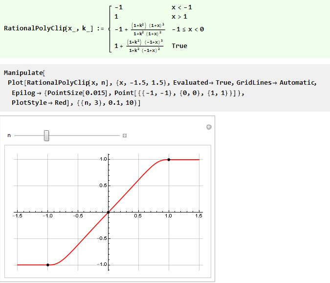
Thus, we can rewrite the previous function with stiffness control using only a rational 3-order polynomial:
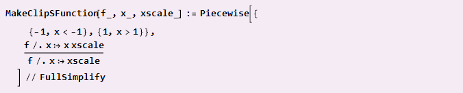
In order not to specify piecewise continuous functions each time, we can define an auxiliary function that will do it itself, taking the donor function as an input as input.
If our function already has a diagonal symmetry and is aligned to the center of coordinates (like a sine wave), then you can simply do
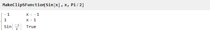
Usage example:
If you need to collect from pieces, as in the case of a parabola, and the center of coordinates determines the docking points, the formula will be slightly more complicated:
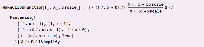
Usage example:
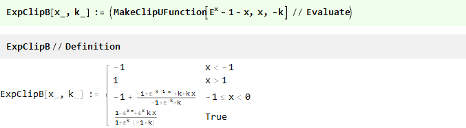
Absolutely any function can be a donor for this task, you just need to provide it with inflection points. Take, for example, the exponent shifted down by one:
Previously, to ensure the required inflection at zero, we squared the function. But you can go the other way - for example, to sum up with another function, the derivative of which at point zero is opposite in sign with the derivative of the exponent. For example, -x:
Depending on which side we take the curve, the final form of the function will depend. Now, using the previously defined auxiliary function and selecting one of the parties, we get:
Or
And now we can compare them on one chart:
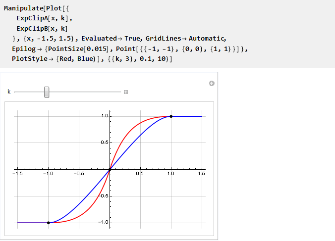
It is seen that as k → 0, they tend to coincide; and since we cannot directly calculate their values, since we obtain the division by zero, we use the limit:
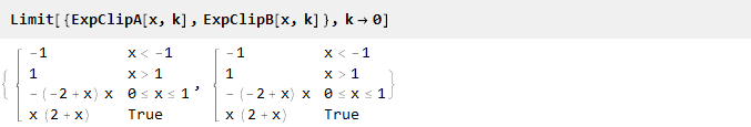
And we got the piecewise function already known to us from the parabola.
So far, we have considered only symmetric functions. However, there are cases when we do not need symmetry - for example, to simulate distortion when sounding tube amplifiers.
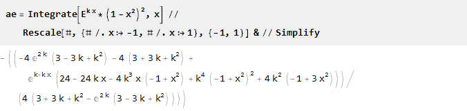
Take the exponent and multiply it by an inverted parabola in the square - to get the intersection with the x-axis at the points -1 and 1, and at the same time to ensure the smoothness of the second derivative; parameterization is also possible through the scaling of the exponent argument:
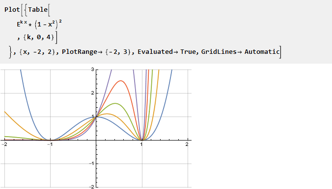
Find the primitive and scale it:
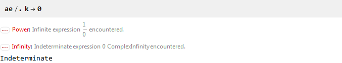
Since for k = 0 we get the division by zero:
Then we will additionally find the limit
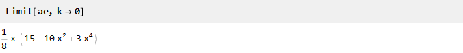
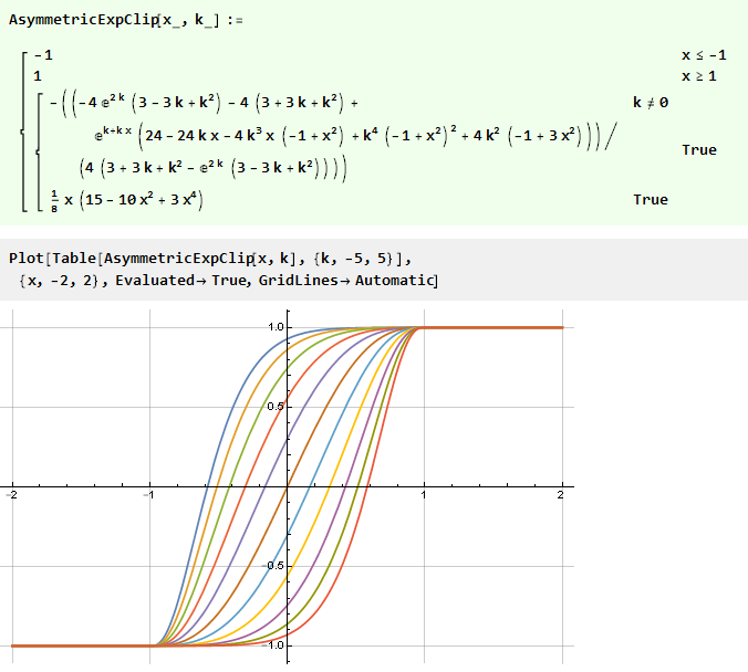
which is a smooth polynomial of the 3rd order already known to us. Combining everything into one function, we get
Instead of initially designing an asymmetric function, you can go the other way - use the finished symmetric, but “distort” the value of this function with the help of an additional function of the curve defined on the interval {-1,1}.
Consider, for example, hyperbole:
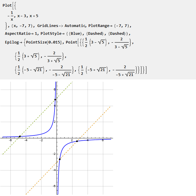
Considering its segment in different scales, you can adjust the degree of curvature in both directions. How to find this segment? Based on the graph, one could look for the intersection of the hyperbola with the straight line. However, since such an intersection does not always exist, this creates some difficulties. Therefore, we will go the other way.
To begin with, add scaling factors to the hyperbola:

then we will make a system of equations defining the conditions for passing the hyperbola through the given points - and solving it will give us the coefficients of interest:
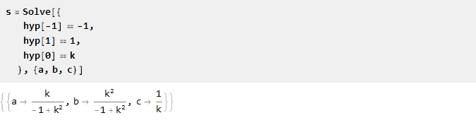
Now we substitute the solution into the original formula and simplify:
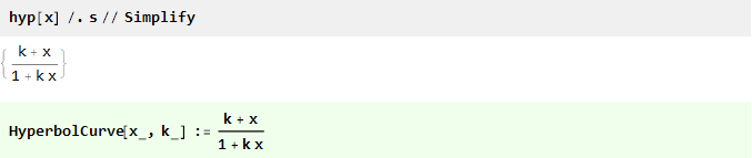
Let's see what we have, depending on the parameter k:
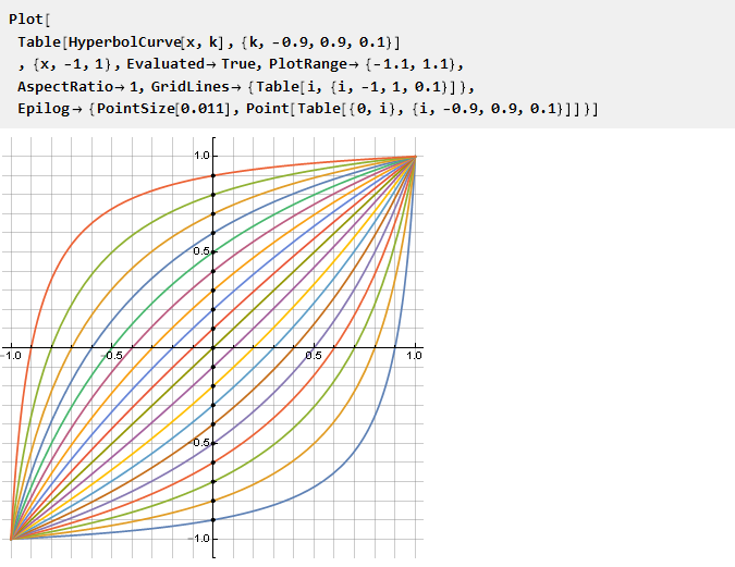
It is noteworthy that for k = 0, the formula collapses in a natural way at x and no special situations occur - although with reference to the initial hyperbola, this is equivalent to a segment of zero length, moreover, to two at once. No less noteworthy is that the inverse of it is the same function, but with a negative parameter k:

Now we can use it to modify an arbitrary function of the constraint, and the parameter k will thus define the intersection point with the y-axis:
Similarly, one can construct curves from other functions, for example, a power function with a variable base:
Or the reverse of it is logarithmic:
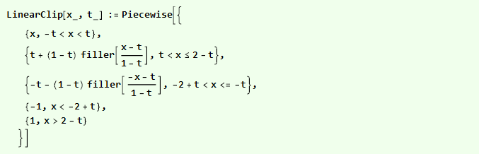
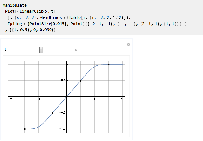
We may want to have a guaranteed linear interval for a function on a certain interval. It is logical to organize the introduction of a straight line into a piecewise continuous function,
empty places in which it is necessary to fill with some function. Obviously, for a smooth docking with a linear segment, its first derivative should be equal to one; and all subsequent (if possible) zero. In order not to not display such a function anew, we can take it ready and adapt it for this task. You can also notice that the extreme points are a little further than one — this is necessary to maintain the slope of the linear section.
Take the PolySoft function derived earlier and shift it so that in the center of coordinates we get one:
From its properties, it follows that the n-1 of the subsequent derivatives at points 0 and 2 will be zero:
Now we integrate it:
The function was shifted down relative to the x-axis. Therefore, it is necessary to add a constant (equal to the value of the function at the point 0) in order to combine the coordinate centers:
Here we have a zero in degree n. It has not declined, since the value of zero to the power of zero is not defined; we can remove it manually, but we can clearly indicate with simplification that n is greater than zero here:
Check in any case. The value at points 0 and 2 for all n:

Derivatives at the edges of the interval (for a polynomial of order 5):
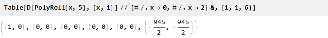
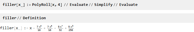
As you can see, the function was rather cumbersome. In order not to drag it and not over-complicate the calculations, we will further manipulate with a particular polynomial, for example of the 4th order:
And now you can fill it with free space:
Check:
Sometimes it may be the need for functions that tend to the unit, but do not reach it. Wikipedia suggests several well-known solutions:
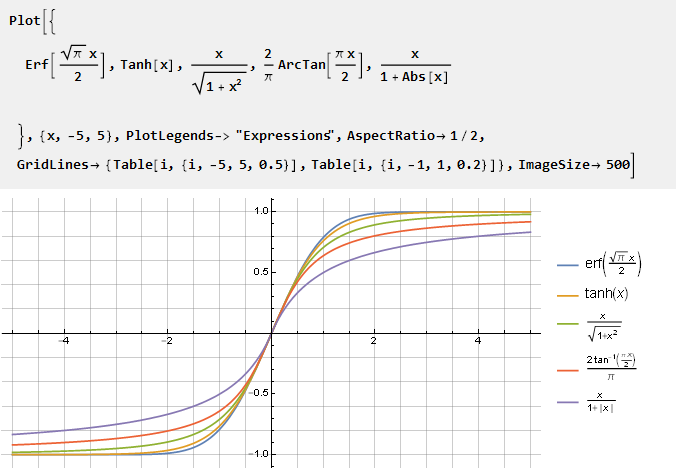
Since these functions of the unit do not reach, it is more convenient to normalize them by the derivative in the center of coordinates.
We can modify the form of such a function through their argument with the help of some diagonally symmetric function, for example:
This function, by the way, is also the inverse of itself, i.e.

And, with reference to arctangent as an example, we get
which, in particular, with the parameter k = 1 will give us the Guderman function .
As we see, with this approach, undesirable kinks can be obtained, therefore, it is more preferable to control the constraint stiffness directly through the property of the function itself. Consider several such functions with a parameter, the output of which is omitted for brevity.
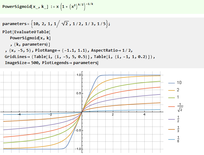
From power function:
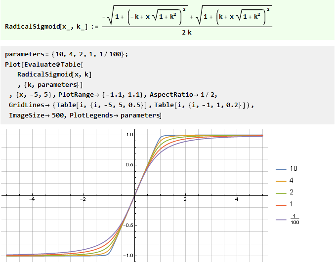
From the sum of two v-shaped functions with an offset:
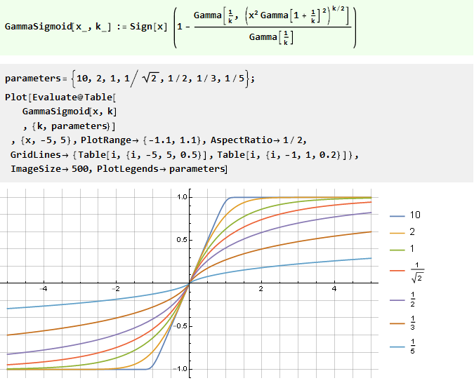
From the generalized error function:
Integrating a rational polynomial:
Interestingly, its special case is arctangent:
Building functions of this kind can be an exciting exercise, during which both simple and complex, beautiful and not so great formulas will be obtained. It may seem that all of them are very similar to each other and there is no need for such a variety. This is not necessarily the case.
The difference may be more visible in other scales - for example, logarithmic. In addition to the tasks indicated in the header, similar functions can be used in other tasks - mixing signals, when a smooth attenuation of one signal is combined with a smooth growth of another, or building acoustic filters - and then the difference will be perceived by ear, or to build gradients - and then the difference will be perceived by eye. In addition, they can also be used as donors for other, more complex functions — for example, window functions.
In conclusion, it is worth clarifying a few more points.
All functions here were defined in the range from -1 to 1. In case another range is needed (for example, from 0 to 1), it can easily be recalculated either manually:
Or using the built-in scaling function:
And to facilitate the export of the formulas in the program code, the CForm function can be useful:
The original Mathematica document can be downloaded here .
Notes:
[1] A true mathematician will certainly be able to strictly prove (or disprove) this statement.
[2] in the standard course of mathematical analysis, hypergeometric functions are not considered.
[3] this overload is defined only for a character unit; a unit in floating point format (for example, when plotting a chart) will not be recognized.
The simplest implementation of the constraint is to force it to a certain value when a certain level is exceeded. For example, for a sinusoid with increasing amplitude, it will look like this:
')
The role of the limiter here is the Clip function, whose argument is the input signal and the parameters of the limit, and the result of the function is the output signal.
Let's look at the graph of the Clip function separately:
It shows that while we do not exceed the limits, the output value is equal to the input value and the signal does not change; if the output value is exceeded, the output value does not depend in any way and remains at the same level. In fact, we have a piecewise continuous function made up of three others: y = -1, y = x and y = 1, selected depending on the argument, and equivalent to the following record:
The transition between functions is quite dramatic; and looks tempting to make it smoother. Mathematically, this sharpness is due to the fact that the derivatives of the functions at the junction points do not coincide. This is easy to see by plotting the derivative of the Clip function:
Thus, to ensure the smoothness of the constraint function, it is necessary to ensure the equality of the derivatives at the docking points. And since the extreme functions of our constants, the derivatives of which are equal to zero, then the derivatives of the constraint function at the junction points must also be zero. Next, we will consider several such functions that provide smooth docking.
Sinus
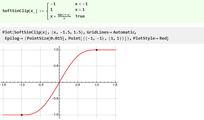
The simplest thing is to use the sin function on the interval from -pi / 2 to pi / 2, at the boundaries of which the values of the derivative are zero by definition:
It is only necessary to scale the arguments so that the unit is projected onto Pi / 2. Now we can define the actual limiting function:
And build its schedule:
Since the limits of the limitation are strictly defined here, the limitation is defined by scaling the input signal followed by (if necessary) reverse scaling.
There is also no situation in which the input signal is transmitted to the output without distortion - the lower the gain level, the lower the level of distortion due to the limitation - but the signal is distorted anyway.
The effect of the gain parameter on signal distortion can be seen in dynamics:
More smoothness
Let's look at the derivative of our function:
It already has no discontinuities in the values, but there are discontinuities in the derivative (the second, if we take it from the original function). In order to eliminate it, you can go the opposite way - first form a smooth derivative, and then integrate it to obtain the desired function.
The easiest way to zero the derived points -1 and 1 is to simply square the function - all negative values of the function will become positive and, accordingly, there will be excesses at the intersection points of the function with zero.
Find the primitive:
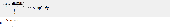
It now remains to scale it along the ordinate axis. For this we find its value at point 1:
And we divide it into it (yes, it is here that this elementary multiplication by 2, but not always the case):
Thus, the final restriction function will take the form:
Go to polynomials
Using trigonometric functions in some cases can be somewhat wasteful. Therefore, we will try to build the function we need, while remaining within the framework of elementary mathematical operations.
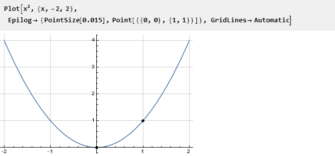
Consider a parabola:
Since it already has an inflection point at zero, we can use the same part on the interval {0,1} for docking with constants. For negative values, you need to move it down and to the left:
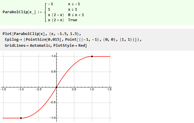
and for positive ones - to reflect vertically and horizontally:
And our function with a parabola will look like:
Complicate things a little
Let's return to our parabola, turn it over and move it up one unit:
This will be a derivative of our function. To make it smoother at the docking points, squared, thus nullifying the second derivative:
We integrate and scale:
We get an even smoother function:
More smoothness god smoothness
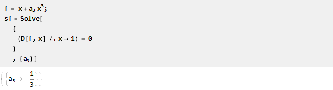
Here we will try to achieve smoothness at the docking points for even higher derivatives. To do this, first define the function as a polynomial with unknown coefficients, and try to find the coefficients themselves by solving a system of equations.
Let's start with the 1st derivative:
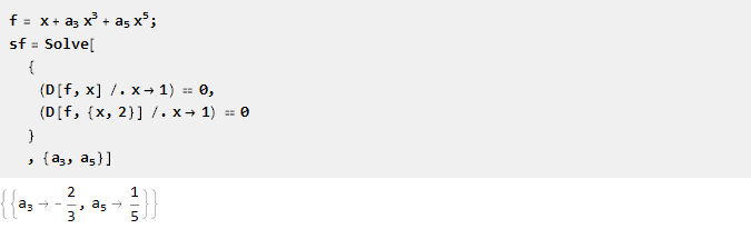
2nd:
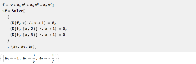
3rd:
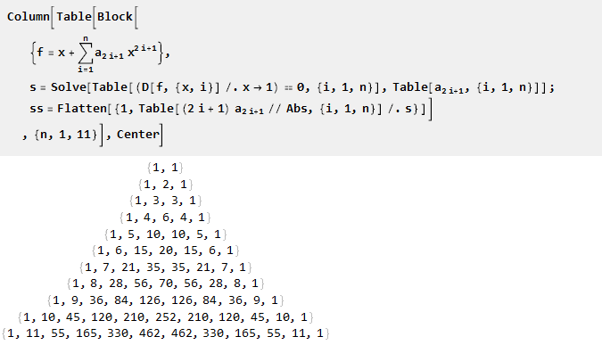
All these coefficients look as if they have some kind of logic. We write down the factors, multiplying them by the value of the degree at x; and in order not to write the same thing every time, we automate the process of finding coefficients:
It looks like the binomial coefficients. We make a bold assumption that this is what they are, and based on this, we write the generalized formula:
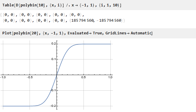
Check:
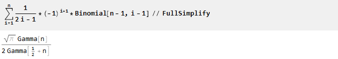
It looks like the truth [1] . It remains only to calculate the scale factor to bring the edges to unity:
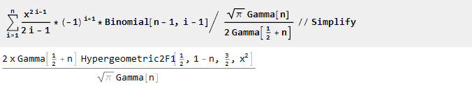
And after scaling and simplifying, we find that our knowledge of mathematics is somewhat outdated [2] :
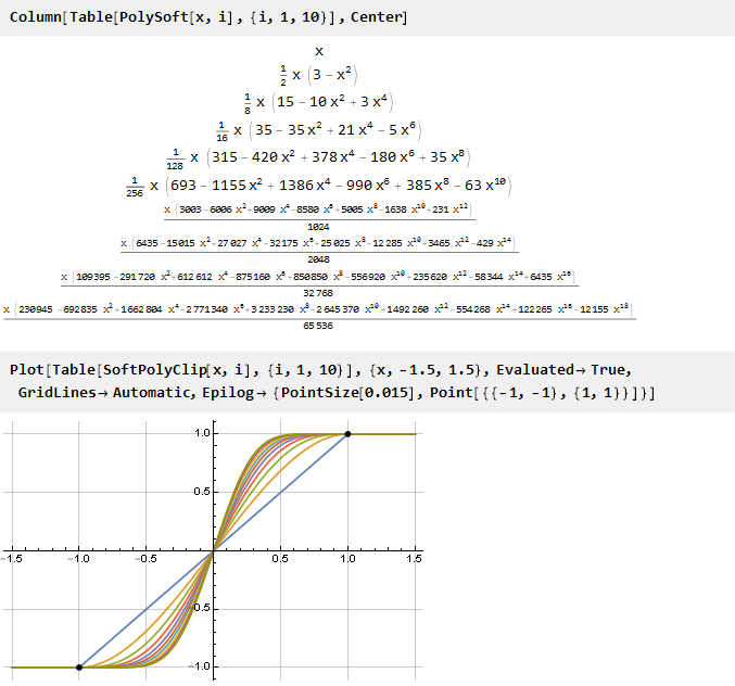
Thus, we have obtained a generating function of order n, in which the n-1 first derivatives will be equal to zero:
Let's see what happened:
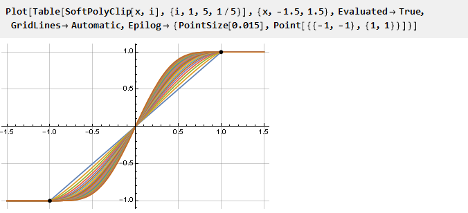
And since our generalized formula turned out to be continuous, if you wish, you can use non-integer parameter values:
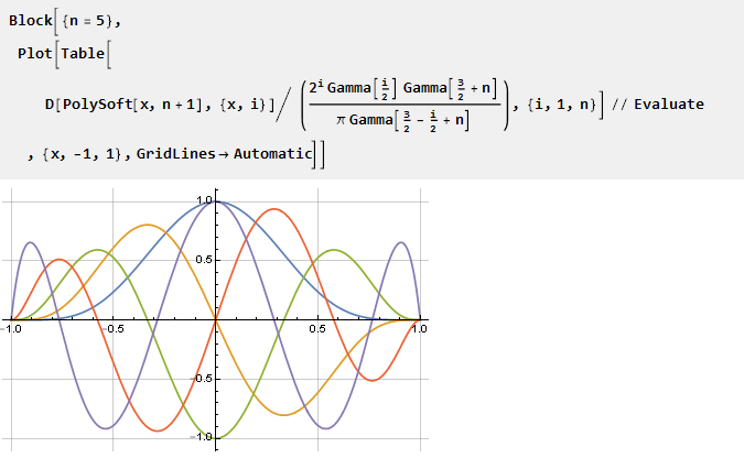
You can also build graphs of derivatives reduced to the same scale:
Add stiffness
It would be tempting to be able to adjust the degree of "stiffness" of the constraint.
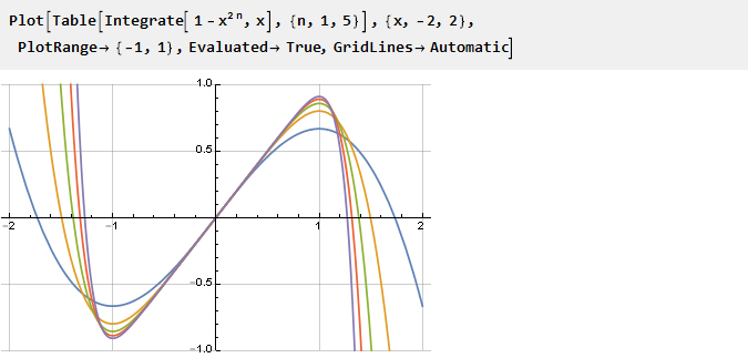
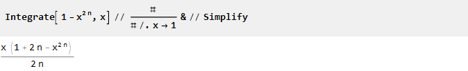
Let us return to our inverted parabola and add the coefficient at degree x:
The greater the n, the more our derivative is “square”, and its primitive is, respectively, sharp:
We calculate the antiderivative and adjust the scale:
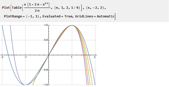
Now let's try to set the fractional step for the parameter:
As we see, in the negative part, not for all n there is a correct solution, but in the right (positive) part, the conditions we need are still met — so for negative values we can simply use it in an inverted form with a reversed argument. And since the domain of definition of the parameter is no longer limited to positive integers, it is possible to simplify the formula by replacing 2n with n:
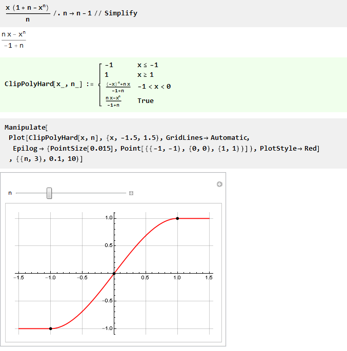
And replacing n with n-1, you can make the formula a little more beautiful:
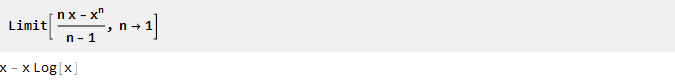
Since when n is equal to unity, we get the division by zero, we will try to find the limit:
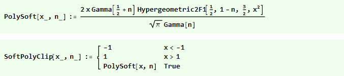
The limit is found, which means that now you can define [3] a function for n equal to 1 and consider it for all n large zero:
If we initially square our inverted parabola, we get an even smoother function:
And we can compare them on one chart:
Rationalize it
Let's look at the following function:
It appeared not by chance.
If you remove the unit from it, x 2 will be reduced and just x will remain, that is, the inclined line. Thus, the smaller the value of x, the greater the influence of the unit in the denominator, creating the curvature we need. And considering this function at different scales, one can control the degree of this curvature:
Thus, we can rewrite the previous function with stiffness control using only a rational 3-order polynomial:
Automate it
In order not to specify piecewise continuous functions each time, we can define an auxiliary function that will do it itself, taking the donor function as an input as input.
If our function already has a diagonal symmetry and is aligned to the center of coordinates (like a sine wave), then you can simply do
Usage example:
If you need to collect from pieces, as in the case of a parabola, and the center of coordinates determines the docking points, the formula will be slightly more complicated:
Usage example:
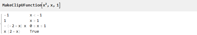
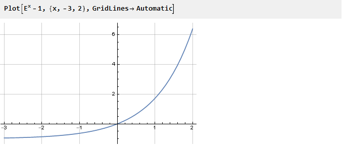
Let's go to the exhibitor
Absolutely any function can be a donor for this task, you just need to provide it with inflection points. Take, for example, the exponent shifted down by one:
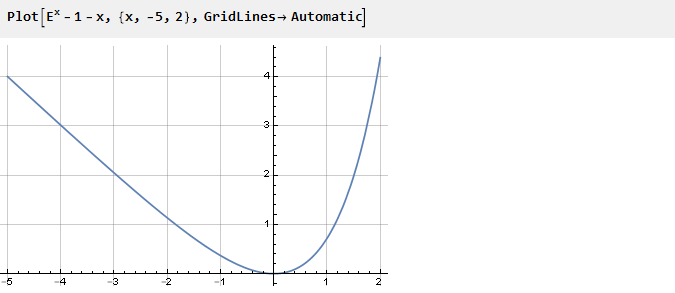
Previously, to ensure the required inflection at zero, we squared the function. But you can go the other way - for example, to sum up with another function, the derivative of which at point zero is opposite in sign with the derivative of the exponent. For example, -x:
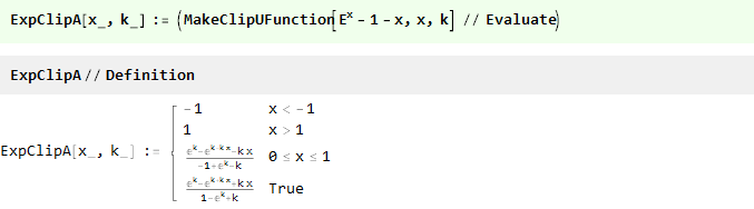
Depending on which side we take the curve, the final form of the function will depend. Now, using the previously defined auxiliary function and selecting one of the parties, we get:
Or
And now we can compare them on one chart:
It is seen that as k → 0, they tend to coincide; and since we cannot directly calculate their values, since we obtain the division by zero, we use the limit:
And we got the piecewise function already known to us from the parabola.
Breaking symmetry
So far, we have considered only symmetric functions. However, there are cases when we do not need symmetry - for example, to simulate distortion when sounding tube amplifiers.
Take the exponent and multiply it by an inverted parabola in the square - to get the intersection with the x-axis at the points -1 and 1, and at the same time to ensure the smoothness of the second derivative; parameterization is also possible through the scaling of the exponent argument:
Find the primitive and scale it:
Since for k = 0 we get the division by zero:
Then we will additionally find the limit
which is a smooth polynomial of the 3rd order already known to us. Combining everything into one function, we get
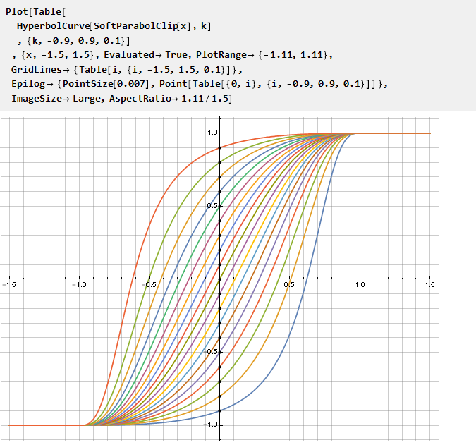
Instead of initially designing an asymmetric function, you can go the other way - use the finished symmetric, but “distort” the value of this function with the help of an additional function of the curve defined on the interval {-1,1}.
Consider, for example, hyperbole:
Considering its segment in different scales, you can adjust the degree of curvature in both directions. How to find this segment? Based on the graph, one could look for the intersection of the hyperbola with the straight line. However, since such an intersection does not always exist, this creates some difficulties. Therefore, we will go the other way.
To begin with, add scaling factors to the hyperbola:
then we will make a system of equations defining the conditions for passing the hyperbola through the given points - and solving it will give us the coefficients of interest:
Now we substitute the solution into the original formula and simplify:
Let's see what we have, depending on the parameter k:
It is noteworthy that for k = 0, the formula collapses in a natural way at x and no special situations occur - although with reference to the initial hyperbola, this is equivalent to a segment of zero length, moreover, to two at once. No less noteworthy is that the inverse of it is the same function, but with a negative parameter k:
Now we can use it to modify an arbitrary function of the constraint, and the parameter k will thus define the intersection point with the y-axis:
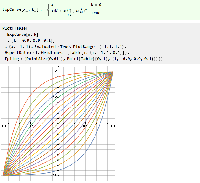
Similarly, one can construct curves from other functions, for example, a power function with a variable base:
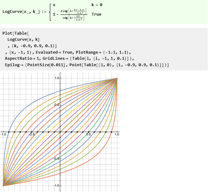
Or the reverse of it is logarithmic:
Need more accuracy
We may want to have a guaranteed linear interval for a function on a certain interval. It is logical to organize the introduction of a straight line into a piecewise continuous function,
empty places in which it is necessary to fill with some function. Obviously, for a smooth docking with a linear segment, its first derivative should be equal to one; and all subsequent (if possible) zero. In order not to not display such a function anew, we can take it ready and adapt it for this task. You can also notice that the extreme points are a little further than one — this is necessary to maintain the slope of the linear section.
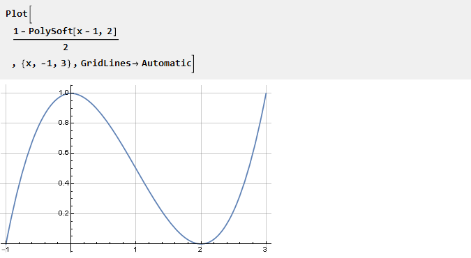
Take the PolySoft function derived earlier and shift it so that in the center of coordinates we get one:
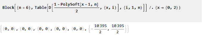
From its properties, it follows that the n-1 of the subsequent derivatives at points 0 and 2 will be zero:
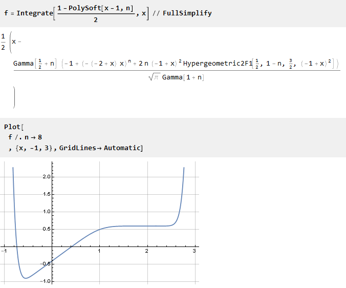
Now we integrate it:
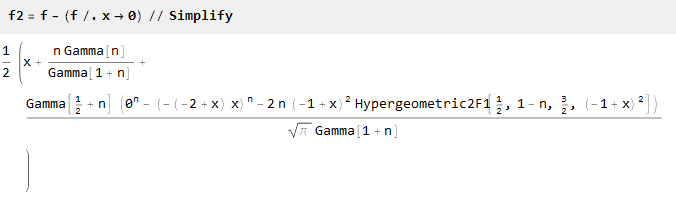
The function was shifted down relative to the x-axis. Therefore, it is necessary to add a constant (equal to the value of the function at the point 0) in order to combine the coordinate centers:
Here we have a zero in degree n. It has not declined, since the value of zero to the power of zero is not defined; we can remove it manually, but we can clearly indicate with simplification that n is greater than zero here:
Check in any case. The value at points 0 and 2 for all n:
Derivatives at the edges of the interval (for a polynomial of order 5):
As you can see, the function was rather cumbersome. In order not to drag it and not over-complicate the calculations, we will further manipulate with a particular polynomial, for example of the 4th order:
And now you can fill it with free space:
Check:
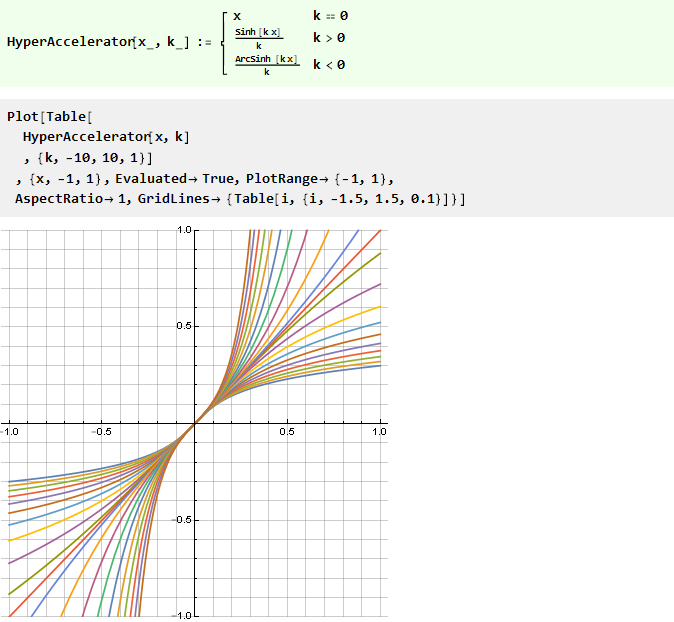
We go to infinity
Sometimes it may be the need for functions that tend to the unit, but do not reach it. Wikipedia suggests several well-known solutions:
Since these functions of the unit do not reach, it is more convenient to normalize them by the derivative in the center of coordinates.
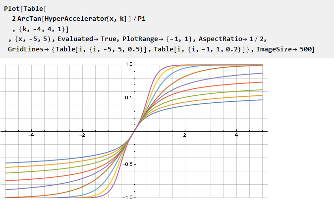
We can modify the form of such a function through their argument with the help of some diagonally symmetric function, for example:
This function, by the way, is also the inverse of itself, i.e.
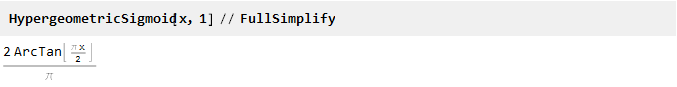
And, with reference to arctangent as an example, we get
which, in particular, with the parameter k = 1 will give us the Guderman function .
As we see, with this approach, undesirable kinks can be obtained, therefore, it is more preferable to control the constraint stiffness directly through the property of the function itself. Consider several such functions with a parameter, the output of which is omitted for brevity.
From power function:
From the sum of two v-shaped functions with an offset:
From the generalized error function:
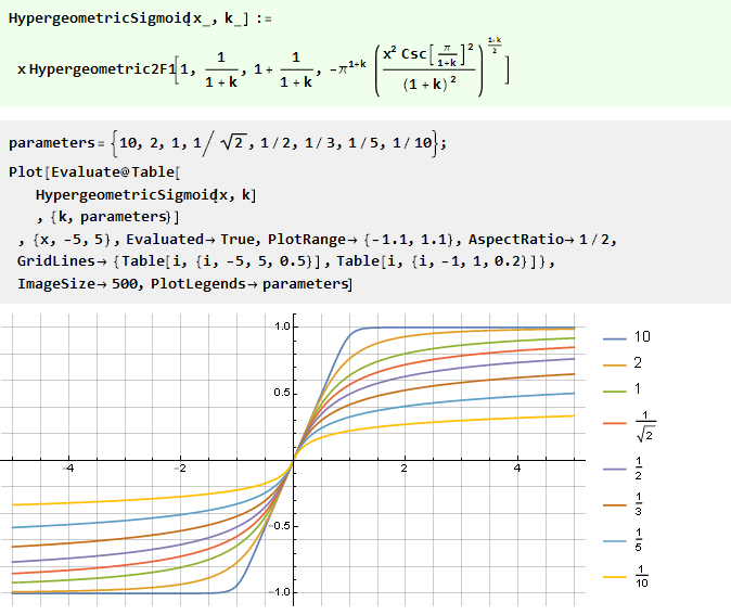
Integrating a rational polynomial:
Interestingly, its special case is arctangent:
Conclusion
Building functions of this kind can be an exciting exercise, during which both simple and complex, beautiful and not so great formulas will be obtained. It may seem that all of them are very similar to each other and there is no need for such a variety. This is not necessarily the case.
The difference may be more visible in other scales - for example, logarithmic. In addition to the tasks indicated in the header, similar functions can be used in other tasks - mixing signals, when a smooth attenuation of one signal is combined with a smooth growth of another, or building acoustic filters - and then the difference will be perceived by ear, or to build gradients - and then the difference will be perceived by eye. In addition, they can also be used as donors for other, more complex functions — for example, window functions.
In conclusion, it is worth clarifying a few more points.
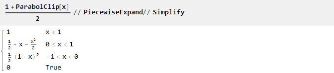
All functions here were defined in the range from -1 to 1. In case another range is needed (for example, from 0 to 1), it can easily be recalculated either manually:
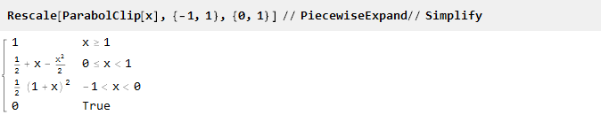
Or using the built-in scaling function:
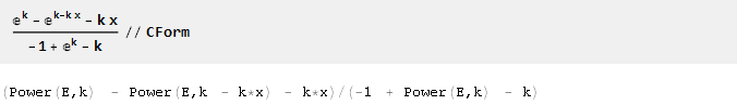
And to facilitate the export of the formulas in the program code, the CForm function can be useful:
The original Mathematica document can be downloaded here .
Notes:
[1] A true mathematician will certainly be able to strictly prove (or disprove) this statement.
[2] in the standard course of mathematical analysis, hypergeometric functions are not considered.
[3] this overload is defined only for a character unit; a unit in floating point format (for example, when plotting a chart) will not be recognized.
Source: https://habr.com/ru/post/424615/
All Articles