Learn OpenGL. Lesson 6.2 - Physically-Based Rendering. Analytical light sources

In the previous lesson we gave an overview of the basics of implementing a physically plausible rendering model. This time we will move from theoretical calculations to a specific implementation of the render with the participation of direct (analytical) light sources: point, directional or projector type.


First, let's refresh the expression for calculating the reflectivity from the previous lesson:

$$

$$L_o (p, \ omega_o) = \ int \ limits _ {\ Omega} (k_d \ frac {c} {\ pi} + \ frac {DFG} {4 (\ omega_o \ cdot n) (\ omega_i \ cdot n) }) L_i (p, \ omega_i) n \ cdot \ omega_i d \ omega_i$$

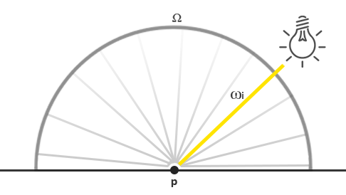
For the most part, we have already dealt with the components of this formula, but the question remains as to how exactly to represent the irradiance value, which represents the total energy brightness ( radiance ) $$$L$the whole scene. We agreed that the energy brightness $$$L$(in terms of computer graphics terminology) is considered as a radiant flux ratio ( radiant flux ) $$$\ phi$(radiation energy of the light source) to the value of the solid angle $$$\ omega$. In our case, the solid angle $$$\ omega$we have assumed infinitely small, and therefore the energy brightness gives an idea of ​​the radiation flux for each individual ray of light (its direction).

How to link these calculations with the lighting model that we know from previous lessons? First, imagine that a single point source of light is given (which radiates uniformly in all directions) with a radiation flux given as the RGB triad (23.47, 21.31, 20.79). The radiant intensity ( radiant intensity ) of such a source is equal to its radiation flux in all directions. However, having considered the problem of determining the color of a specific point $$$p$on the surface, it can be seen that from all possible directions of the incidence of light in the hemisphere $$$\ Omega$only vector $$$w_i$will clearly come from the light source. Since only one light source is given, represented by a point in space, for all other possible directions of light falling to a point $$$p$energy brightness will be zero:

Now, if we temporarily ignore the law of light attenuation for a given source, it turns out that the energy brightness for the incident beam of this source light remains unchanged wherever we place the source (scaling the luminosity based on the cosine of the angle of incidence $$$\ phi$also does not count). In total, the point source maintains the radiation power constant regardless of the viewing angle, which is equivalent to accepting the magnitude of the radiation force equal to the initial radiation flux in the form of a constant triad (23.47, 21.31, 20.79).

However, the calculation of the energy brightness is also based on the coordinate of the point $$$p$At least any physically reliable light source demonstrates attenuation of the radiation power with increasing distance from the point to the source. The orientation of the surface should also be taken into account, as can be seen from the initial expression for luminosity: the result of calculating the radiation power should be multiplied by the value of the scalar multiplication of the surface normal vector $$$n$and the radiation falling vector $$$w_i$.

To rewrite the above: for a direct point source of light, the emission function $$$L$determines the color of the incident light taking into account the attenuation at a given distance from the point $$$p$and given the scaling factor $$$n \ cdot w_i$but only for a single ray of light $$$w_i$getting to a point $$$p$- essentially the only vector connecting the source and point. In the form of source code, this is interpreted as follows:

vec3 lightColor = vec3(23.47, 21.31, 20.79); vec3 wi = normalize(lightPos - fragPos); float cosTheta = max(dot(N, Wi), 0.0); float attenuation = calculateAttenuation(fragPos, lightPos); vec3 radiance = lightColor * attenuation * cosTheta; 

If you close your eyes to slightly changed terminology, this piece of code should remind you of something. Yes, yes, this is all the same code for calculating the diffuse component in the lighting model known to us. For direct illumination, the energy brightness is determined by a single vector to the source of light, because the calculation is carried out in a manner so similar as we still know.

I note that this statement is true only in the framework of the assumption that the point source of light is infinitely small and is represented by a point in space. When modeling a volume source, its luminosity will differ from zero in a variety of directions, and not just on a single ray.

For other light sources emitting radiation from a single point, the energy brightness is calculated in the same way. For example, a directional light source has a constant direction. $$$w_i$and does not use attenuation, and the projector source exhibits varying radiant power, depending on the direction of the source.

Here we return to the value of the integral $$$\ int$on the surface of the hemisphere $$$\ Omega$. Since we know in advance the positions of all the particular points of the light sources involved in the shading, we do not need to try to solve the integral. We can directly calculate the total irradiance provided by this number of light sources, since the only direction for each source affects the energy brightness of the surface.

As a result, the PBR calculation for direct light sources is quite simple, since it all comes down to a sequential enumeration of the sources involved in the illumination. Later, a component of the environment will appear in the lighting model, which we will work on in the lighting-based image -based lesson ( Image-Based Lighting , IBL ). There is no way out of assessing the integral, since the light in such a model falls from a multitude of directions.

PBR surface model

Let's start with a fragment shader that implements the PBR model described above. First, we define the input data required for shading:

 #version 330 core out vec4 FragColor; in vec2 TexCoords; in vec3 WorldPos; in vec3 Normal; uniform vec3 camPos; uniform vec3 albedo; uniform float metallic; uniform float roughness; uniform float ao; 

Here you can see the usual input data calculated using the simplest vertex shader, as well as a set of uniforms describing the characteristics of the object's surface.

Next, at the very beginning of the shader code, let's perform calculations, so familiar from the implementation of the Blinna-Phong lighting model:

 void main() { vec3 N = normalize(Normal); vec3 V = normalize(camPos - WorldPos); [...] } 

Direct lighting

The example for this lesson contains only four point light sources that clearly set the irradiance of the scene. To satisfy the expression of reflectivity, we iteratively go through each light source, calculate the individual energy brightness and sum up this contribution, modulating along the way the BRDF value and the angle of incidence of the light beam. You can imagine this iteration as a solution of the integral over the surface $$$\ Omega$only for analytical light sources.

So, we first calculate the values ​​for each source:

 vec3 Lo = vec3(0.0); for(int i = 0; i < 4; ++i) { vec3 L = normalize(lightPositions[i] - WorldPos); vec3 H = normalize(V + L); float distance = length(lightPositions[i] - WorldPos); float attenuation = 1.0 / (distance * distance); vec3 radiance = lightColors[i] * attenuation; [...] 

Since the calculations are carried out in linear space (we perform gamma correction at the end of the shader), the more physically correct damping law is used according to the inverse square of the distance:

Let the law of the inverse square and more physically correct, in order to better control the nature of the attenuation it is quite possible to use the already familiar formula containing constant, linear and quadratic terms.

Further, for each source, we also calculate the value of the Mirror Cook-Torrance BRDF:

$$

$$\ frac {DFG} {4 (\ omega_o \ cdot n) (\ omega_i \ cdot n)}$$

The first step is to calculate the ratio between the specular and diffuse reflection, or, in other words, the ratio between the amount of reflected light to the amount of light refracted by the surface. From the previous lesson we know what the Fresnel coefficient calculation looks like:

 vec3 fresnelSchlick(float cosTheta, vec3 F0) { return F0 + (1.0 - F0) * pow(1.0 - cosTheta, 5.0); } 

The Fresnel-Schlick approximation expects the input parameter F0 , which shows the degree of reflection of the surface at zero angle of incidence of light , i.e. the degree of reflection, if you look at the surface along the normal from top to bottom. The value of F0 varies depending on the material and acquires a colored tint for metals, as can be seen by viewing the catalogs of PBR materials. For the process of metallic workflow (the authoring process for PBR materials, dividing all materials into classes of dielectrics and conductors), it is assumed that all dielectrics look quite reliably at a constant value of F0 = 0.04 , while for metal surfaces, F0 is set based on the surface albedo. In the form of code:

 vec3 F0 = vec3(0.04); F0 = mix(F0, albedo, metallic); vec3 F = fresnelSchlick(max(dot(H, V), 0.0), F0); 

As you can see, for strictly non-metallic surfaces, F0 is set to 0.04. But at the same time, it can smoothly change from this value to the magnitude of the albedo on the basis of the surface “metallicity” indicator. This indicator is usually presented in the form of a separate texture (hence, the metallic workflow is taken from here, approx. Lane ).

Having received $$$F$it remains for us to calculate the value of the normal distribution function $$$D$and geometry functions $$$G$:

Function code for an analytical lighting case:

 float DistributionGGX(vec3 N, vec3 H, float roughness) { float a = roughness*roughness; float a2 = a*a; float NdotH = max(dot(N, H), 0.0); float NdotH2 = NdotH*NdotH; float num = a2; float denom = (NdotH2 * (a2 - 1.0) + 1.0); denom = PI * denom * denom; return num / denom; } float GeometrySchlickGGX(float NdotV, float roughness) { float r = (roughness + 1.0); float k = (r*r) / 8.0; float num = NdotV; float denom = NdotV * (1.0 - k) + k; return num / denom; } float GeometrySmith(vec3 N, vec3 V, vec3 L, float roughness) { float NdotV = max(dot(N, V), 0.0); float NdotL = max(dot(N, L), 0.0); float ggx2 = GeometrySchlickGGX(NdotV, roughness); float ggx1 = GeometrySchlickGGX(NdotL, roughness); return ggx1 * ggx2; } 

An important difference from that described in the theoretical part : here we directly pass the roughness parameter to all the functions mentioned. This is done to allow each of the functions to modify the original roughness value in their own way. For example, Disney's research, reflected in the Epic Games engine, showed that the lighting model gives more visually correct results if the square of the roughness is used in the geometry function and the normal distribution function.

By setting all the functions, you can directly get the NDF and G values:

 float NDF = DistributionGGX(N, H, roughness); float G = GeometrySmith(N, V, L, roughness); 

In total, we have on hand all the values ​​to calculate the entire Cook-Torrance BRDF:

 vec3 numerator = NDF * G * F; float denominator = 4.0 * max(dot(N, V), 0.0) * max(dot(N, L), 0.0) + 0.001; vec3 specular = numerator / denominator; 

Please note that we limit the denominator to a minimum value of 0.001 to prevent division by zero, in cases of zeroing the scalar product.

We now proceed to the calculation of the contribution of each source to the equation of reflectivity. Since the fresnel coefficient directly represents a variable $$$K_s$, then F can be used to denote the source's contribution to the specular reflection of the surface. Of magnitude $$$K_s$can be obtained and the refractive index $$$K_d$:

 vec3 kS = F; vec3 kD = vec3(1.0) - kS; kD *= 1.0 - metallic; 

Since we consider the value of kS to represent the amount of light energy reflected by the surface, then subtracting it from the unit, we obtain the residual energy of light kD refracted by the surface. In addition, since the metals do not refract light and do not have the diffuse component of the reradiated light, the kD component will be modulated so as to be zero for a completely metallic material. After these calculations, we will have all the data for calculating the reflectivity provided by each of the light sources:

 const float PI = 3.14159265359; float NdotL = max(dot(N, L), 0.0); Lo += (kD * albedo / PI + specular) * radiance * NdotL; } 

The total value Lo , or outgoing energy brightness, is essentially a solution to the expression of reflectivity, i.e. result of integration over the surface $$$\ Omega$. In this case, we do not need to try to solve the integral in a general form for all possible directions, since in this example there are only four sources of light that affect the processed fragment. That is why all the "integration" is limited to a simple cycle of existing light sources.

It remains only to add the similarity of the background lighting component to the results of the calculation of the direct light source and the resulting color of the fragment is ready:

 vec3 ambient = vec3(0.03) * albedo * ao; vec3 color = ambient + Lo; 

Linear space and HDR rendering

Until now, we assumed that all calculations are carried out in a linear color space, and therefore we used gamma correction as the final chord in our shader. Carrying out calculations in linear space is extremely important for correct PBR modeling, since the model requires linearity of all input data. Try not to ensure the linearity of any of the parameters and the result of shading will be incorrect. In addition, it would be nice to set the characteristics of light sources close to real sources: for example, the color of their radiation and the energy brightness can freely vary within wide limits. As a consequence, Lo can quite easily take large values, but will inevitably fall under the cutoff in the interval [0., 1.] due to the low dynamic range ( LDR ) of the frame buffer by default.

To avoid losing HDR values, it is necessary to perform tone mapping before gamma correction:

 color = color / (color + vec3(1.0)); color = pow(color, vec3(1.0/2.2)); 

Here, the already familiar Reinhard operator is used, which allows preserving a wide dynamic range in the conditions of highly varying irradiance of different parts of the image. Since here we do not use a separate shader for post-processing, the described operations can be added simply to the end of the shader code.


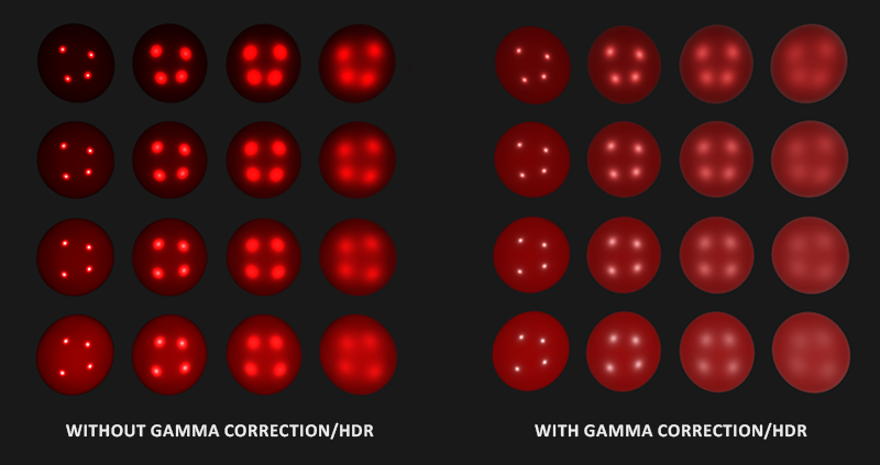
I repeat that for correct PBR modeling it is extremely important to remember and take into account the peculiarities of working with linear color space and HDR render. Neglect of these aspects will lead to incorrect calculations and visually unaesthetic results.

PBR shader for analytical lighting

So, together with the last strokes in the form of tonal compression and gamma correction, it remains only to transfer the final color of the fragment to the output of the fragment shader and the PBR code of the shader for direct illumination can be considered complete. Finally, let's take a look at the whole code of the main () function of this shader:

 #version 330 core out vec4 FragColor; in vec2 TexCoords; in vec3 WorldPos; in vec3 Normal; //   uniform vec3 albedo; uniform float metallic; uniform float roughness; uniform float ao; //   uniform vec3 lightPositions[4]; uniform vec3 lightColors[4]; uniform vec3 camPos; const float PI = 3.14159265359; float DistributionGGX(vec3 N, vec3 H, float roughness); float GeometrySchlickGGX(float NdotV, float roughness); float GeometrySmith(vec3 N, vec3 V, vec3 L, float roughness); vec3 fresnelSchlickRoughness(float cosTheta, vec3 F0, float roughness); void main() { vec3 N = normalize(Normal); vec3 V = normalize(camPos - WorldPos); vec3 F0 = vec3(0.04); F0 = mix(F0, albedo, metallic); //    vec3 Lo = vec3(0.0); for(int i = 0; i < 4; ++i) { //        vec3 L = normalize(lightPositions[i] - WorldPos); vec3 H = normalize(V + L); float distance = length(lightPositions[i] - WorldPos); float attenuation = 1.0 / (distance * distance); vec3 radiance = lightColors[i] * attenuation; // Cook-Torrance BRDF float NDF = DistributionGGX(N, H, roughness); float G = GeometrySmith(N, V, L, roughness); vec3 F = fresnelSchlick(max(dot(H, V), 0.0), F0); vec3 kS = F; vec3 kD = vec3(1.0) - kS; kD *= 1.0 - metallic; vec3 numerator = NDF * G * F; float denominator = 4.0 * max(dot(N, V), 0.0) * max(dot(N, L), 0.0); vec3 specular = numerator / max(denominator, 0.001); //       Lo float NdotL = max(dot(N, L), 0.0); Lo += (kD * albedo / PI + specular) * radiance * NdotL; } vec3 ambient = vec3(0.03) * albedo * ao; vec3 color = ambient + Lo; color = color / (color + vec3(1.0)); color = pow(color, vec3(1.0/2.2)); FragColor = vec4(color, 1.0); } 

I hope that after getting acquainted with the theoretical part and with today's analysis of the expression of reflectivity, this listing will no longer look daunting.

We use this shader in a scene containing four point light sources, an unlimited number of spheres, the surface characteristics of which will change the degree of their roughness and metallicity along the horizontal and vertical axes, respectively. At the output we get the following picture:


Metallicity varies from zero to one from the bottom up, and the roughness is similar, but from left to right. It becomes clear that changing only these two characteristics of the surface it is already possible to set a wide range of materials.

The full source code is here .

PBR and texturing

Expand our surface model by transferring characteristics in the form of textures. Thus, we will be able to provide fragmentary control over the parameters of the surface material:

 [...] uniform sampler2D albedoMap; uniform sampler2D normalMap; uniform sampler2D metallicMap; uniform sampler2D roughnessMap; uniform sampler2D aoMap; void main() { vec3 albedo = pow(texture(albedoMap, TexCoords).rgb, 2.2); vec3 normal = getNormalFromNormalMap(); float metallic = texture(metallicMap, TexCoords).r; float roughness = texture(roughnessMap, TexCoords).r; float ao = texture(aoMap, TexCoords).r; [...] } 

Note that the surface albedo texture is usually created by artists in the sRGB color space, so in the code above we return the texel color to the linear space so that it can be used in further calculations. Depending on how the artists create the texture containing the ambient occlusion map data, you may also need to bring it into linear space. Metallicity and roughness maps are almost always created in linear space.

The use of textures instead of fixed surface parameters in combination with the PBR algorithm gives a significant increase in visual accuracy compared to the previously used lighting algorithms:


The full code of the texturing example is here , and the textures used are here (along with the background shading texture). I draw your attention to the fact that strongly metallic surfaces appear darkened under direct illumination conditions, since the contribution of diffuse reflection is small (in the limit it is completely absent). Their shading becomes more correct only when taking into account the mirror reflection of light from the environment, which we will do in the next lessons.

At the moment, the result obtained may not be as impressive as some PBR demonstrations - yet we have not yet implemented an image-based lighting system ( IBL ). Nevertheless, our render is now considered to be based on physical principles and, even without IBL, it shows a more reliable picture than before.