Evenly distribute points over a sphere in pytorch and tensorflow

This text is written for those who are interested in deep learning, who want to use the different methods of the pytorch and tensorflow libraries to minimize the function of many variables, who are interested in learning how to turn a sequentially running program into numpy vectorized matrix calculations. And you can also learn how to make a cartoon of the data rendered using PovRay and vapory.

Whence the task

Everyone minimizes their functionality (c) Anonymous data scientist

In one of the previous publications of our blog , namely in the item "Rake No. 6", it was told about the DSSM technology, which allows you to convert text into vectors. To find such a mapping, we need to find the coefficients of linear transformations that minimize the rather complicated loss function. Understanding what happens when learning such a model is difficult because of the large dimension of the vectors. To develop an intuition that allows you to choose the right optimization method and set the parameters of this method, you can consider a simplified version of this task. Now let the vectors be in our usual three-dimensional space, then they are easy to draw. And the loss function will be the potential for repulsing points from each other and attraction to the unit sphere. In this case, the solution of the problem will be the uniform distribution of points on the sphere. The quality of the current solution is easy to assess by eye.

So, we will look for a uniform distribution over a sphere of a given amount. $$$n$points. Such a distribution is necessary acoustics in order to understand in which direction to launch a wave in a crystal. To the communications operator - to learn how to place satellites in orbit to achieve the best quality of communication. Meteorologist - to accommodate weather monitoring stations.

For some $$$n$The problem is solved easily . For example, if $$$n = 8$, we can take a cube and its vertices will be the answer to the problem. Also we are lucky if $$$n$will be equal to the number of vertices of the icosahedron, dodecahedron, or other Plato body. Otherwise, the task is not so simple.

For a sufficiently large number of points there is a formula with empirically selected coefficients , a few more options - here , here , here , and here . But there is a more universal, albeit a more complex solution , to which this article is devoted.

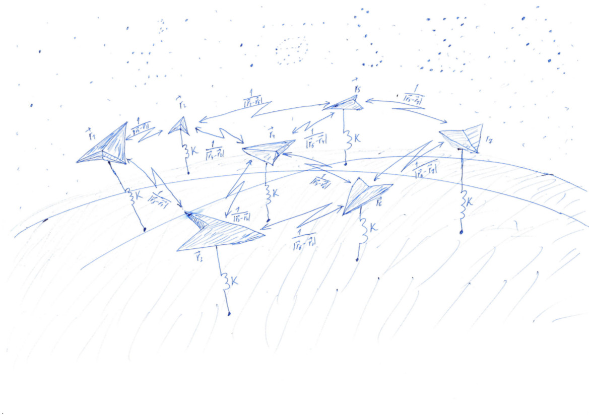
We solve a problem that is very similar to the Thomson problem ( wiki ). Scatter $$$n$points by chance, and then force them to attract some kind of surface, for example, to a sphere, and repel each other. Attraction and repulsion are determined by the function - potential. At the minimum value of the potential function, the points will lie on the sphere most evenly.

This task is very similar to the learning process of machine learning (ML) models, in which the loss function is minimized. But a data scientist usually looks at how a single number decreases, and we can watch the change in the picture. If everything works out for us, we will see how the points randomly placed inside the cube with side 1 will disperse over the surface of the sphere:

Schematically, the algorithm for solving the problem can be represented as follows. Each point located in three-dimensional space corresponds to a row of matrix $$$X$. The loss function is calculated using this matrix. $$$L$whose minimum value corresponds to a uniform distribution of points on the sphere. The minimum value is found using the pytorch and tensorflow , which allow to calculate the loss function gradient over the matrix $$$X$and go down to the minimum using one of the methods implemented in the library: SGD, ADAM, ADAGRAD, etc.

We consider the potential

Due to its simplicity, expressiveness and ability to serve as an interface to libraries written in other languages, Python is widely used to solve machine learning problems. Therefore, the code examples in this article are written in Python. To perform fast matrix calculations, we will use the numpy library. To minimize the function of many variables - pytorch and tensorflow.

Randomly scatter points in a cube with side 1. Let us have 500 points, and elastic interaction is 1000 times more significant than electrostatic:

 import numpy as np n = 500 k = 1000 X = np.random.rand(n, 3) 

This code generated a matrix $$$X$by size $$$3 \ times n$filled with random numbers from 0 to 1:

We assume that each row of this matrix corresponds to one point. And in three columns recorded coordinates $$$x, y, z$all our points.

Potential of elastic interaction of a point with the surface of a single sphere $$$u_1 = k \ cdot (1 - r) ^ 2/2$. Potential electrostatic interaction points $$$p$and $$$q$- $$$u_2 = 1 / | r_p - r_q |$. The full potential consists of the electrostatic interaction of all pairs of points and the elastic interaction of each point with the surface of the sphere:

$$

$$U (x_1, ..., x_n) = \ sum \ limits _ {p = 1} ^ {n - 1} \ sum \ limits _ {q = p + 1} ^ {n} \ frac 1 {\ left | \ vec {x_p} - \ vec {x_q} \ right | } + k \ cdot \ sum \ limits _ {p = 1} ^ n \ left (1 - | \ vec {x_p} | \ right) ^ 2 \ rightarrow \ min$$

In principle, one can calculate the value of the potential using this formula:

 L_for = 0 L_for_inv = 0 L_for_sq = 0 for p in range(n): p_distance = 0 for i in range(3): p_distance += x[p, i]**2 p_distance = math.sqrt(p_distance) L_for_sq += k * (1 - p_distance)**2 #     ,     for q in range(p + 1, n): if q != p: pq_distance = 0 for i in range(3): pq_distance += (x[p, i] - x[q, i]) ** 2 pq_distance = math.sqrt(pq_distance) L_for_inv += 1 / pq_distance #      L_for = (L_for_inv + L_for_sq) / n print('loss =', L_for) 

But there is a little trouble. For a measly 2000 points, this program will run for 2 seconds. It will be much faster if we calculate this value using vectorized matrix calculations. Acceleration is achieved both through the implementation of matrix operations using the “fast” languages ​​of fortran and C, and through the use of vectorized processor operations, which allow performing an action on a large amount of input data in one clock cycle.

Look at the matrix $$$S = X \ cdot X ^ T$. It has many interesting properties and is often found in calculations related to the theory of linear classifiers in ML. So, if we assume that in the row of the matrix $$$X$with indexes $$$p$and $$$q$three-dimensional space vectors are written $$$\ vec {r _ p}, \ vec {r_q}$, the matrix $$$S$will consist of the scalar products of these vectors. Such vectors $$$n$pieces, then the dimension of the matrix $$$S$equals $$$n \ times n$.

On the diagonal of the matrix $$$S$are squares of lengths of vectors $$$\ vec {r_p}: s_ {p p} = r_p ^ 2$. Knowing this, let's consider the full potential of interaction. Let's start with the calculation of two auxiliary matrices. In one diagonal of the matrix $$$S$will be repeated in rows, in the other - in columns.

Now let's look at the value of the expression p_roll + q_roll - 2 * S

Element with indexes $$$(p, q)$sq_dist matrix equals $$$r_p ^ 2 + r_q ^ 2 - 2 \ cdot (\ vec {r_p}, \ vec {r_q}) = (\ vec {r_p} - \ vec {r_q}) ^ 2$. That is, we have a matrix of squares of distances between points.

Electrostatic repulsion on a sphere

dist = np.sqrt(sq_dist) - matrix of distances between points. We need to calculate the potential, taking into account the repulsion of points between themselves and the attraction to the sphere. Let's put on the diagonal of the unit and replace each element with the opposite one (just don’t think that we drew the matrix!): rec_dist_one = 1 / (dist + np.eye(n)) . It turned out the matrix, on the diagonal of which there are units, the other elements - the potentials of electrostatic interaction between the points.

We now add the quadratic potential of attraction to the surface of the unit sphere. Distance from the surface of the sphere $$$(1 - r)$. Square it up and multiply by $$$k$which defines the relation between the role of electrostatic repulsion of particles and the attraction of a sphere. Total k = 1000 , all_interactions = rec_dist_one - torch.eye(n) + (d.sqrt() - torch.ones(n))**2 . The long-awaited loss function, which we will minimize: t = all_interactions.sum()

A program that calculates potential using the numpy library:

 S = X.dot(XT) #    pp_sq_dist = np.diag(S) #  p_roll = pp_sq_dist.reshape(1, -1).repeat(n, axis=0) #     q_roll = pp_sq_dist.reshape(-1, 1).repeat(n, axis=1) #     pq_sq_dist = p_roll + q_roll - 2 * S #      pq_dist = np.sqrt(pq_sq_dist) #    pp_dist = np.sqrt(pp_sq_dist) #      surface_dist_sq = (pp_dist - np.ones(n)) ** 2 #       rec_pq_dist = 1 / (pq_dist + np.eye(n)) - np.eye(n) #      L_np_rec = rec_pq_dist.sum() / 2 #     L_np_surf = k * surface_dist_sq.sum() #       L_np = (L_np_rec + L_np_surf) / n #   ,     print('loss =', L_np) 

Here things are a little better - 200 ms for 2000 points.

Use pytorch:

 import torch pt_x = torch.from_numpy(X) # pt_x -   tensor   pytorch pt_S = pt_x.mm(pt_x.transpose(0, 1)) # mm - matrix multiplication pt_pp_sq_dist = pt_S.diag() pt_p_roll = pt_pp_sq_dist.repeat(n, 1) pt_q_roll = pt_pp_sq_dist.reshape(-1, 1).repeat(1, n) pt_pq_sq_dist = pt_p_roll + pt_q_roll - 2 * pt_S pt_pq_dist = pt_pq_sq_dist.sqrt() pt_pp_dist = pt_pp_sq_dist.sqrt() pt_surface_dist_sq = (pt_pp_dist - torch.ones(n, dtype=torch.float64)) ** 2 pt_rec_pq_dist = 1/ (pt_pq_dist + torch.eye(n, dtype=torch.float64)) - torch.eye(n, dtype=torch.float64) L_pt = (pt_rec_pq_dist.sum() / 2 + k * pt_surface_dist_sq.sum()) / n print('loss =', float(L_pt)) 

And finally, tensorflow:

 import tensorflow as tf tf_x = tf.placeholder(name='x', dtype=tf.float64) tf_S = tf.matmul(tf_x, tf.transpose(tf_x)) tf_pp_sq_dist = tf.diag_part(tf_S) tf_p_roll = tf.tile(tf.reshape(tf_pp_sq_dist, (1, -1)), (n, 1)) tf_q_roll = tf.tile(tf.reshape(tf_pp_sq_dist, (-1, 1)), (1, n)) tf_pq_sq_dist = tf_p_roll + tf_q_roll - 2 * tf_S tf_pq_dist = tf.sqrt(tf_pq_sq_dist) tf_pp_dist = tf.sqrt(tf_pp_sq_dist) tf_surface_dist_sq = (tf_pp_dist - tf.ones(n, dtype=tf.float64)) ** 2 tf_rec_pq_dist = 1 / (tf_pq_dist + tf.eye(n, dtype=tf.float64)) - tf.eye(n, dtype=tf.float64) L_tf = (tf.reduce_sum(tf_rec_pq_dist) / 2 + k * tf.reduce_sum(tf_surface_dist_sq)) / n glob_init = tf.local_variables_initializer() #     with tf.Session() as tf_s: #     glob_init.run() #   res, = tf_s.run([L_tf], feed_dict={tf_x: x}) #   print(res) 

Compare the performance of these three approaches:

N	python	numpy	pytorch	tensorflow
2000	4.03	0.083	1.11	0.205
10,000	99	2.82	2.18	7.9

Vectorized calculations give a gain of more than one and a half decimal orders relative to the code in pure python. The pytorch boiler plate is visible: it takes a lot of time to compute a small volume, but it almost doesn’t change as the computation increases.

Visualization

Nowadays, data can be visualized by means of a huge number of packages, such as Matlab, Wolfram Mathematica, Maple, Matplotlib, etc., etc. There are a lot of complex functions in these packages that do complex things. Unfortunately, if you are faced with a simple, but non-standard task, you find yourself unarmed. My favorite solution in this situation is povray. This is a very powerful program that is usually used to create photorealistic images, but it can be used as a "visualization assembler". Usually, no matter how complex the surface that you want to display, it is enough to ask povray to draw spheres with centers lying on this surface.

Using the vapory library, you can create a povray scene right in python, render it and look at the result. Now it looks like this:

The picture was obtained as follows:

 import vapory from PIL import Image def create_scene(moment): angle = 2 * math.pi * moment / 360 r_camera = 7 camera = vapory.Camera('location', [r_camera * math.cos(angle), 1.5, r_camera * math.sin(angle)], 'look_at', [0, 0, 0], 'angle', 30) light1 = vapory.LightSource([2, 4, -3], 'color', [1, 1, 1]) light2 = vapory.LightSource([2, 4, 3], 'color', [1, 1, 1]) plane = vapory.Plane([0, 1, 0], -1, vapory.Pigment('color', [1, 1, 1])) box = vapory.Box([0, 0, 0], [1, 1, 1], vapory.Pigment('Col_Glass_Clear'), vapory.Finish('F_Glass9'), vapory.Interior('I_Glass1')) spheres = [vapory.Sphere( [float(r[0]), float(r[1]), float(r[2])], 0.05, vapory.Texture(vapory.Pigment('color', [1, 1, 0]))) for r in x] return vapory.Scene(camera, objects=[light1, light2, plane, box] + spheres, included=['glass.inc']) for t in range(0, 360): flnm = 'out/sphere_{:03}.png'.format(t) scene = create_scene(t) scene.render(flnm, width=800, height=600, remove_temp=False) clear_output() display(Image.open(flnm)) 

From the heap of files, animated gif is collected using ImageMagic:

 convert -delay 10 -loop 0 sphere_*.png sphere_all.gif 

On github, you can see the working code, fragments of which are shown here. In the second article I will talk about how to run the minimization of the functional, so that the points come out of the cube and evenly spread over the sphere.