Optimization of prices in offline retail

This article opens the retail cycle. The idea of ​​using analytics in retail can be portrayed as such a marketing circle:

The main idea, at first glance, of a useless picture is to show that the analyst allows you to predict the consequences of making certain business decisions, based on the subsequent change in consumer demand. And the better we understand the demand, aggregating information from different channels, the better we will predict the result. In short, the picture of the ideal world, and each goes to this world in its own way.

Today we will talk about pricing analytics in offline retail.

Introduction

Wiki provides a concise definition of pricing . From the point of view of the company, pricing is another tool that allows you to manage the demand for goods / services and, accordingly, the company's KPIs. Why not take advantage of the achievements of digitalization and data science to help the company place prices more efficiently.
Typical retail pricing of goods is as follows:

• Products for which the price is limited due to government regulation: tobacco, some drugs. In this case, usually do not bother and put the maximum allowable price.
• Goods indicators for the buyer. They are rigidly priced from competitors on the basis of rules like "our price = competitor price - 2%" (KVI, first price, locomotives, etc.)
• The rest of the goods ( back basket ), which each price according to its capabilities. It is about them today that we will talk about how to set the price for these goods in the best possible way. There remains on average about half of the revenue.

Closer to the point

Briefly, the whole process of price optimization can be described in the following steps:

1. Build a model of consumer demand for historical data
2. We collect the pricing rules of the business (about them below) and turn them into mathematical optimization constraints
3. We run the optimization for a given KPI (margin, revenue, units) and get the best prices

It doesn't look very difficult, but the details begin.

For simplicity, consider the process of optimizing prices from the end. If the first two items are fulfilled (i.e., demand patterns are built and pricing rules are formalized), the third is a purely technical step (of course, if you know which KPI should be optimized). Optimization methods invented many for different tasks . In the end, you can just go over the price grid and find the best one, even though this is not the approach of real Jedi.

The second point is a separate and very difficult task of collecting rules for automating pricing. There is not a lot of analytics and mathematics here, but the main problem is to formalize and agree on the rules that are in the mind of several dozen Nikolaev Sergeyevich. Fortunately, there is a more or less well-established set of rule templates from which to start:

• Margin is not lower / not higher than N [%] or N [rub.]
• Price change no more than N [%] or N [rub.]
• The price within the price cluster is the same.
• The price within the product lines is the same.
• The price per unit volume is cheaper for more goods.
• Price cannot be lower / higher than N [%], relative to competitors
• STM is cheaper than brand by N [%]
• The price format is ##. 00, # 9.95 (yes, such prices are still very much loved, and not only in Russia)

Well, here is the most interesting first point - building a model of consumer demand.

Model type and data

The model should be built taking into account the fact that it will be used for further optimization. Those. tree busts are good when you have a small number of “product / store” pairs, but try optimizing by boostering 10,000,000 “product / store” pairs for a 5 hour night window (besides, have you seen how tree ensembles take prices into account?).

In this area, linear models are still being controlled. As practice shows, a well-tuned linear model is not inferior to the average boosting “the date Satanist saentista. But even if the linear regression slightly concedes to another model - it’s not so bad, because The final task is to determine the best price, and not the most accurate forecast.

Our task is to get models (or models) that will predict the demand for each product in each store. Typical data that is needed for this is a history of sales, a history of balances, a history of prices, a history of promo. Optionally, you can add other data such as competitors' prices, weather, loyalty data, or transactional data. In this case, usually in good condition there is only a sales history. Remains may be jumping because of write-offs, theft and just problems taking into account (there are cases when there may be -0.4 cans of green peas on the remnants, so think what that means). The history of prices and promo in general is a separate story - they are hard to find in the depths of ERP (and sometimes they are simply not there). Of course, it is possible to recover prices from sales, but this will have an appropriate effect on the quality of modeling and, of course, not for the better.

Small offtop

It is often difficult to explain that analytics can generally help in pricing. Here are two typical cases:

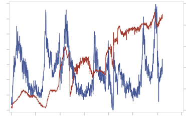
Case 1. Blue shows sales in [pieces] in time, red - price. Here the customer shows us this chart and says: we do not have a classic dependence on price, because the price rises and the demand rises, the price falls and the demand falls. At the end of the article it will be clear what to do in this case (and no - this is not a product of Giffen ).

Here, in addition to the price, additional factors must be taken into account. Such factors can be (not limited to):

• Own prices and prices of competitors
• Promotional events
• Holidays
• Seasonality
• Trends
• Product life cycle
• Inventory

The problem we are solving is to understand how the change in price influences the demand for other known factors.

Case 2. The graph shows the sale of goods in time. It is difficult to find a dependence on the price, if the goods are sold one piece per week.

The answer lies on the surface - it is necessary to aggregate the data to obtain a useful signal.
Let us now analyze these two cases in detail.

Factor and aggregation

So that the model can take into account external factors and be optimized in a reasonable time, let's use linear regression . On the topic “which model is best to use,” not a single dissertation was written, but in practice two very simple models of the following form proved to be well-known:

$$

$$\ log (Sales) = \ alpha + \ beta \ cdot \ log (Price_t) + \ gamma \ cdot Promo_t + \ delta \ cdot Holiday_t + \ ldots$$

$$

$$\ log (Sales) = \ alpha + \ beta \ cdot Price_t + \ gamma \ cdot Promo_t + \ delta \ cdot Holiday_t + \ ldots$$

Let's go ahead and use them.

If there is a lack of data, it is logical to use aggregation. In this case, under the aggregation can be understood the following steps:

• Vertical information pooling (vertical information pooling) - aggregation in the classical sense, for example, to look at sales of goods at the level of the city, rather than a specific store.
• Horizontal information pooling (horizontal information pooling) - the use of econometric models with fixed , random, and mixed effects using panel data.

Once we have decided on the forecasting model and the aggregation method, we can proceed to the decomposition of demand — that is, evaluate the regression coefficients at the most appropriate level of the commodity-geographical hierarchy. At the same time, we believe that all levels below the hierarchy inherit dependencies obtained at higher levels. Often you have to go back to the stage of choosing a model and method of aggregation and try several options for decomposition.

Decomposition of demand consists of the following steps:

1. At the upper levels of the commodity-geographical hierarchy, we estimate seasonal, cyclical, and trend components using time series methods.
2. At average levels, we subtract the resulting seasonality, build the very regression model that we talked about above - we estimate the influence of external factors.
3. At the lower levels, we subtract the seasonality and influence of factors. As a result, we have unexplained residues. We call them local trends and again predict time series.

The result of demand decomposition is its own forecasting model for each pair of “goods-store”.

It would seem that all problems have been solved, for each pair of “goods store” they built their linear model, it remains to impose restrictions and send everything to the optimizer. In fact, the main difficulty in demand decomposition is to build the correct hierarchy and determine the optimal levels of regression construction. To do this, we need to build a suitable product and geographical hierarchy. Often, company hierarchies respond to more managerial tasks (for example, financial hierarchy or hierarchy associated with suppliers, etc.). They are poorly suited for the problem of modeling demand, so you need to build your class hierarchy.

To build a product hierarchy, it is necessary to study how the buyer makes the decision to purchase goods. And, asking ourselves this question, we come to a new concept - customer decision tree (Customer Decision Tree, CDT) . It shows which attributes of goods are important for the buyer, and in what sequence they should be located.

In most cases, CDT is based on the attributes of the goods. The lower the CDT level, the stronger the goods replace each other. Category managers can be of great help in building a CDT, since understand their categories well. There are analytical methods for constructing CDT, for example, analysis of the transaction graph. The description of such methods is a separate article.

Building a geographic hierarchy is usually a simpler task. Clustering on the structure of seasonality, the structure of sales categories, and the movements of customers can help here.

An interesting case was in one grocery retailer: the structure of demand differed greatly depending on which side of the major roads there were shops - more vodka, beer and cigarettes were taken in the direction of the region, more cleaning products, children's yoghurts and animal feed were taken in the direction of the center. - it was a stable pattern of consumption.

Having built a separate CDT and geographical hierarchy, we combine them into a commodity-geographical one. Thus, we have built a new hierarchy, which is great for modeling demand.

What is the result

As a result, we built a new hierarchy, which is well suited for demand modeling, and also obtained a sequence of actions that need to be done to build demand models themselves for further optimization. Here is a brief order of building models:

• We estimate seasonality, trend, cyclical components.
  
  • We aggregate data to the level of the commodity-geographical hierarchy, on which we evaluate seasonality, trend and cyclical components.
  • All levels of hierarchies below inherit the resulting values.
• We aggregate data to the level at which we will evaluate the influence of external factors.
• Subtract seasonality and trend
• We evaluate the influence of external factors.
  
  • All levels of hierarchies below inherit the calculated impact estimate from external factors.
• Subtract the obtained values ​​of seasonality and assessment of the influence of external factors at the most detailed level - product / store
• The remains are smoothed and predicted by simple methods. Restoring seasonality, holidays, the effect of promo and prices.

As a result, for each product in each store, we received our own formula:

$$

$$Sales = f (Price, Promo, Seas, Holiday, Inventory, Lcycle, ...)$$

People from business will immediately ask, but how is the mutual influence of goods on each other taken into account? It can be taken into account at the modeling stage in several ways, but here are the two most popular ones:

• Direct method - we take into account the prices of goods, which have the greatest influence on each other in the demand formula:

  
  

  $$

  $$Sales = f (Price, Price_I, Price_K, ...)$$
  
  

• Modeling the share of sales - we forecast sales of the group and the share of each product within the group:

  
  

  $$

  $$Group \ _sales = f (Avg \ _price, Promo_I, Promo_K, ...)$$
  
  

  $$

  $$Item \ _share_I = f (Price_I, Promo_I, Price_K, Promo_K, ...)$$
  
  

Next, the formulas for each pair of “goods store” are sent to the optimizer and get the best prices at the output.

What about that example?

Yes, at first glance, the dependence of demand on price is really absent, set the maximum price and rejoice.
But building a new hierarchy for forecasting, calculating the seasonality at a higher level, subtract it at the level of goods.

Typical dependence of demand on price (the higher the price, the lower the demand). Those. in this case, the effect of seasonality is clearly seen, taking into account which it is immediately obvious that the product is quite elastic.

Conclusion

Optimizing prices is not only beneficial for the company (a few percent of the margin has not disturbed anyone yet), but also interesting. Here there are regressions, optimization, and graph analysis, and all this is in a big wrapper date - there is much to be done for the analyst's soul. But do not forget that demand modeling and price optimization is only a small part of a large business pricing process and, apart from the rest, brings little benefit.

Optimize processes, optimize prices, optimize data storage (after all, Garbage In - Garbage Out) and get great results.