Julia. Acquaintance

Ode to Julia

It is very difficult to convey all the enthusiasm that accompanied the launch of the first programs and the correction of the first errors using this language. Simple and beautiful as Python , a bit like Fortran , convenient work with arrays and graphs, as well as the ability to perform fierce optimization and paralleling even for teapots such as I my classmates. You can work at different levels of abstraction: from high-level programming with dynamic typing, you can descend to assembler commands, that is, here you and Python general accessibility and speed of execution Fortranovskih counters. I can not get rid of the feeling that Mathcad , Scilab and even, God forgive me, C ++ are beginning to fade into my heart.

I found out about the language by accidentally stumbling upon a Habrovo publication , and, as an impressionable student should be, started looking for manuals, preferably in Russian. Since the language had been constantly developing for six years, already scarce sources of information became obsolete, and the excitement began to decrease. But with the beginning of a new laboratory course on modeling physical phenomena with a free choice of programming language, there was still a motivation to begin acquaintance with Julia. In addition, in August, the language "finish the 1.0" .

The following material was planned as an introduction to the language in which all laboratory materials were subsequently written and the training manual was assembled.

Julia is a high-level, high-performance programming language with dynamic typing for mathematical calculations. The syntax is similar to the matlabovo family, the language is written in C , C ++ and Scheme , there is the ability to call Sishny libraries

Installation

Well, everything has finally been established, now at our disposal:

• JuliaPRO Command Prompt - all Yulina's skills directly from the interpreter.
• Juno is a beautiful IDE with a window for graphs and a workspace where you can view the contents of all objects.
• Jupyter - runs the compute kernel in the console, and you can execute the code directly in the browser. (In addition to Julia, there is also a Python)

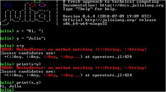
Let's see what this calculator can do ... Unicode support - you can use Cyrillic, hieroglyphs and call pi a Greek letter. You can also not explicitly specify the multiplication between the number and the variable (in this order and without a space):

x = 5+8 2x - 3x + 2x^2 Out: 325 

All the necessary signs are also in place: + =, * =, >> =, etc. (The sign ">>" (bit shift to the right.) Comparison signs:>,> =, <, <=, ==,! =. Inequalities can be combined into chains:

 y = 5 y += 2 4 <= y < 8 Out: true 

Complex numbers available:

 (2-1im)*(4+3im) Out: 11 + 2im 

And functions to work with them:

• real (z) is the real part
• imag (z) - imaginary part
• conj (z) is a complex conjugate number
• abs (z) - module,
• abs2 (z) is the square of the module,
• angle (z) is the argument of a complex number.

You can use rational numbers using "//" and the corresponding functions:

• num (x) is the numerator
• den (x) is the denominator
• float (x) - converts to decimal

 x = 4//6+5//7 Out: 29//21 float(x) Out: 1.380952380952381 

Julia has the ability to control the internal presentation of data:

• typeof (obj) - object type
• typemax (obj) - the maximum number of this type
• typemin (obj) - the minimum
• eps () - machine zero
• BigInt is a big whole
• BigFloat - big float

 q = 3 typemax(q) Out: 9223372036854775807 typeof(q) Out: Int64 BigFloat(2.3^45/6) Out: 3.159376405019356000000000000000000000000000000000000000000000000000000000000e+15 

Functions

A set of special functions

• abs (x) is the modulus of a number
• abs2 (x) is the square of the module,
• sqrt (x) - square root,
• cbrt (x) is the cube root,
• exp (x) is the exponent of a number
• log (x) is the natural logarithm
• log10 (x) is the decimal logarithm
• log (b, x) is the logarithm of x at the base b.
  As well as trigonometric, hyperbolic, Airy, Bessel and many more others.

User functions:

 function () #  end 

The function returns the result of the last expression (Uknul user Mathcad ).

 function cube(x) x^3 end cube(4) Out: 64 

Well, or we will explicitly indicate:

 function myabs(x) if x>=0 return x else return -x end end myabs(-12) Out: 12 

Return values ​​can be assembled into a tuple:

 function cubeandsquare(x) x^3,x^2 end a,b = cubeandsquare(3) print("a = $a, b = $b") Out: a = 27, b = 9 

Functions can accept tuples, default values, keywords. If there are no brackets after the function name, it is treated as a variable and can be assigned to another variable or passed to the function as a parameter. Julia also supports the functional style of writing programs (hello to Lisp)

 function mysin(t;A=1,?=1,?=0) #   -     A*sin(?*t + ?) end x1 = mysin(pi) #   = 0 x2 = mysin(pi*0.5,A = 2) #      x3 = mysin(pi*0.5,? = 0.5) #      print("x1 = $x1, x2 = $x2, x3 = $x3") Out: x1 = 1.2246467991473532e-16, x2 = 2.0, x3 = 0.7071067811865475 

Arrays

As a user of Scilab, I did not even notice the substitution: you can specify an array using the function:

• Array {T} (undef, dims ...) - Array of type T and dimension dims
• zeros (T, dims ...) - Array of zeros
• ones (T, dims ...) - or units
  Indexing starts from one , instead of $ - end , and all necessary operations for matrices are defined (in order to accomplish, say, elementwise addition or multiplication, you need to put a period before the operator).

(Now it’s clear how to insert pictures, but okay ...)

Basic functions:

• det (A) - calculate the determinant
• A ' - transpose matrix
• inv (A) - invert the matrix
• length (A) - the number of elements
• ndims (A) - the number of dimensions
• size (A) - tuple of dimensions
• size (A, n) - dimension in a given direction
• copy (A) - create a copy of the array
• linspace (start, end, step) or
  linspace (beginning: step: end) - creating a one-dimensional array

 A = [1 2 3; 6 5 4; 7 8 9] Out: 3?3 Array{Int64,2}: 1 2 3 6 5 4 7 8 9 A[2,1] Out: 6 A[end] Out: 9 size(A) Out: (3, 3) 

You can select parts of an array by specifying a range of indices along the dimension using the ":" sign.

 m1 = rand(3,2) m2 = reshape(1:2:11, 3,2) Out: 3?2 Base.ReshapedArray{Int64,2,StepRange{Int64,Int64},Tuple{}}: 1 7 3 9 5 11 m3 = [m1 m2] #   (  ) Out: 3?4 Array{Float64,2}: 0.325649 0.701038 1.0 7.0 0.513579 0.620215 3.0 9.0 0.815242 0.805307 5.0 11.0 m5 = [m1; m2] #   (  ) Out: 6?2 Array{Float64,2}: 0.325649 0.701038 0.513579 0.620215 0.815242 0.805307 1.0 7.0 3.0 9.0 5.0 11.0 m3[:, 2:4] Out: 3?3 Array{Float64,2}: 0.701038 1.0 7.0 0.620215 3.0 9.0 0.805307 5.0 11.0 

Here we used rand (), which returns an array of random numbers of a given dimension, and reshape (), which changes the dimension of the array to the specified one.

 for a in A #   a   A end 

or

 for i in eachindex(A) #     i end 

or

 for i = 1 : size(A,n) # n -      (..    ) #     i end 

Charts

To use graphics, you need to download a package to choose from the repository:

• Pkg.add ("Plots")
• Pkg.add ("PyPlot")
• Pkg.add ("Gadfly")
• Pkg.add ("Winston")

Of these, the most popular is Python PyPlot . Modules are connected using a command, for example:

 using PyPlot 

However, let's try Gaston using Gnuplot (swinging separately).
Loading Gaston.jl command

  Pkg.add("Gaston") 

And immediately to the point:

 using Gaston t = 0:0.01:1 plot(t, sin.(2?*5*t))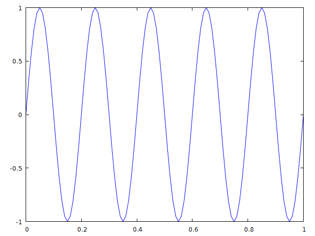 

 plot(t,sin.(2?*5*t),title="A sine wave",xlabel="Time (s)",ylabel="Amplitude",grid="on",linewidth=3,color="blue", yrange="[-1.1:1.1]",marker="ecircle",plotstyle="linespoints",linestyle="-.-")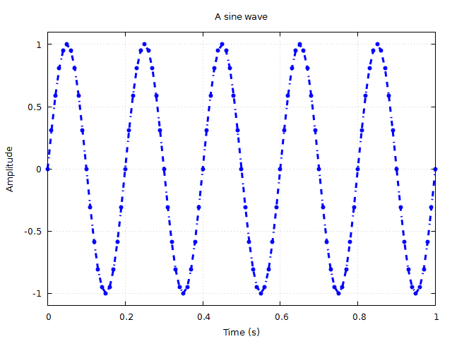 

 plot!(t,cos.(2?*5*t),color="red",linewidth=2) #       

 x = y = -15:0.33:15 surf(x,y,(x,y)->sin.(sqrt.(x.*x+y.*y))./sqrt.(x.*x+y.*y),title="Sombrero",plotstyle="pm3d")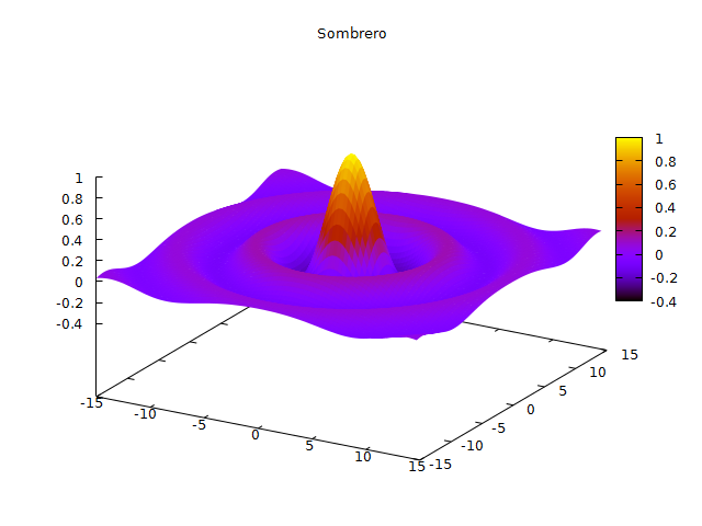 

 x = y = -15:0.33:15 surf(x,y,(x,y)->sin.(sqrt(x.*x+y.*y))./sqrt.(x.*x+y.*y), title="Edge view of a sombrero",plotstyle="pm3d",gpcom="set view 80,20") 

 R = [ x+y for x=0:5:120, y=0:5:120] G = [ x+y for x=0:5:120, y=120:-5:0] B = [ x+y for x=120:-5:0, y=0:5:120] Z = zeros(25,25,3) Z[:,:,1] = R Z[:,:,2] = G Z[:,:,3] = B imagesc(Z,title="RGB Image",clim=[10 200]) 

 histogram(rand(1000),bins=15,norm=1,title="Histogram",yrange="[0:1.6]") 

 y = 1:40 err = Gaston.ErrorCoords(rand(40)) plot(y,err=err,title="Example of error bars",plotstyle="errorbars") 

You can create several graphical windows (does not work in Jupyter ) using the h = figure () command (just insert between plot'ami). To save the graph as an image file, use the commands
set_filename ("name.png") # if not specified, will be displayed
printfigure ("png") # save to file, available PNG, PDF, SVG and GIF
More information on the Gaston package

Conclusion

There are still many graphic packages for every taste and covering almost all needs. Also, auxiliary packages are being developed. Here you have both quantum computing, and bioinformatics, and machine learning, and many more pressing problems like difures and derivatives .

In general, Julia is beautiful, intelligent and very promising, and it is extremely unacceptable to leave her without proper attention.