Anything in MetaPost
What to draw vector images? For me, as for many others, the answer is pretty obvious: most likely in the illustrator. Well or in inkskape. I also thought when I was ordered to draw about eight hundred pictures for a physics textbook. Nothing like that, just black and white technical illustrations with all sorts of blocks, balls, springs, lenses, cars, tractors and so on. It was supposed that the book would be printed in late copy, and I was provided with the files with inserted pictures — sometimes pencil sketches, then scans from other books — and it seemed like a manuscript in some form. In this case, the first thought - to draw in the inkscape - gave way to fantasies on the topic “how to automate everything like this”. For some reason, MetaPost seemed the best option at that moment.
')
The most significant advantage of this solution is that each picture may be a small function of several variables; such a picture is easy, for example, to change in size and fit the stripes to specific unknown circumstances without disturbing important proportions, which is difficult to achieve with more traditional means. And still repeating elements - those balls and springs - can be made to behave much more interesting than the means of “human” vector editors allow.
I wanted to make pictures with shading, like the one found in old books.
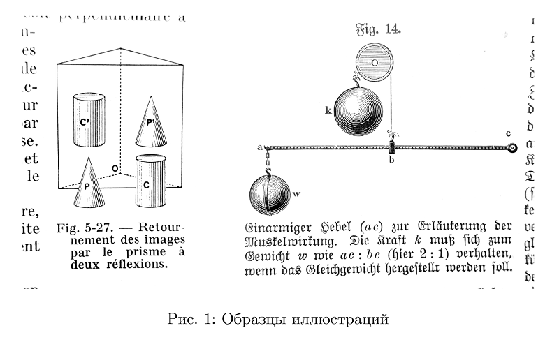
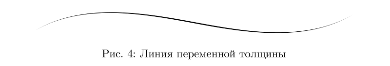
To begin with, it was necessary to get lines of variable thickness. The main difficulty here is to build a curve that is more or less parallel to a given one and, as appropriate, changing the distance to a given one. I relied on the most probably primitive way in which the segments connecting the intermediate points of the Bezier curve are simply transferred in parallel to this distance. With the difference that this distance can vary along the curve.
In most cases, this allows for a tolerable result.
Now, from two such curves you can make a contour of the line of variable thickness.
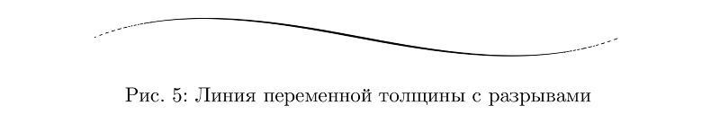
The thickness should be limited to something below, otherwise too thin parts of the lines will be taken on by a raster when printing, and this is usually not very beautiful. One option is to make all the lines, the thickness of which is less than some value, with dashed lines of the same minimum thickness, such that the total amount of paint per unit length corresponds on average to that of the target thickness line. That is, instead of reducing the amount of paint from the sides of the line, begin to gnaw it with transverse stripes.
Now you can draw the balls. These may simply be concentric circles, the thickness of the lines which are determined by the function of the illumination of the ball at the points through which the lines pass.

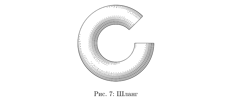
Another convenient primitive is “hoses”: roughly speaking, cylinders that can be bent in every direction. As long as they are of constant section, everything is simple with them.
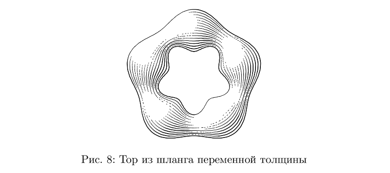
If the thickness changes, it is necessary to change the number of strokes accordingly, while maintaining the average fill density unchanged, as well as to take into account changes in the thickness when calculating the illumination.
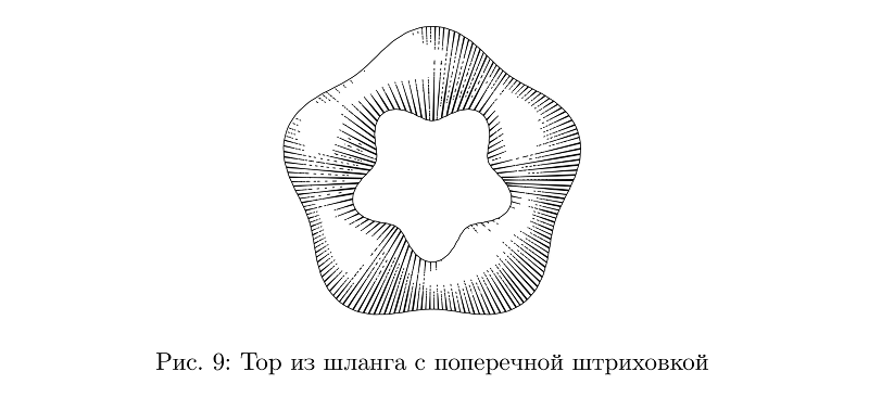
There are more hoses with cross-hatching, but for them to solve the problem of preserving the average filling density turned out to be more difficult, so in many cases they still do not look very good.
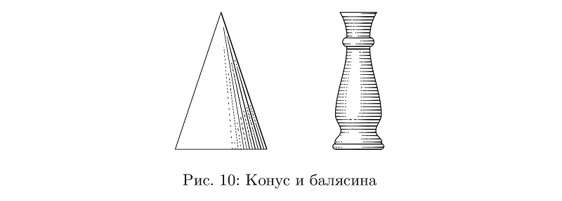
In principle, a lot of things can be made from hoses alone: from cones and cylinders to balusters.
Something from what can be built from such parts is in the library. Let's say a globe is basically a ball.
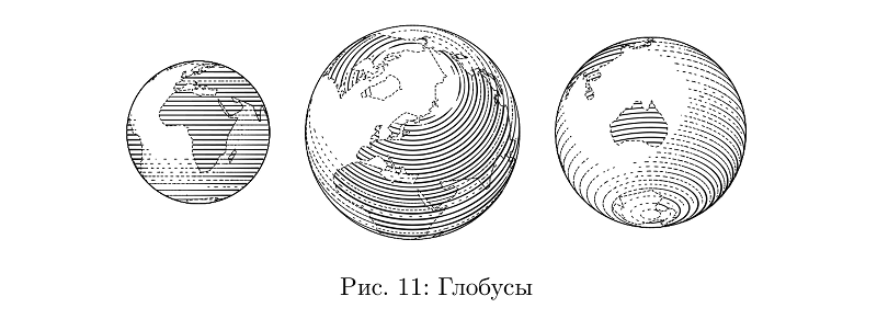
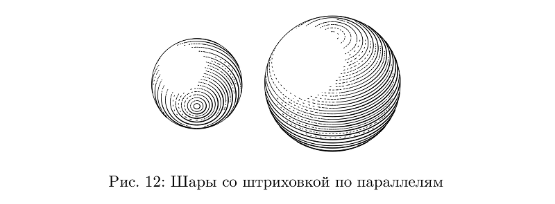
Although not: here the hatching goes along the parallels, and it is even more difficult to control the thickness of the stroke in order to preserve the filling density than in the case of cross-hatching on the hoses, so this is a separate type of ball.
A weight is an uncomplicated construction of two types of hoses of variable thickness.

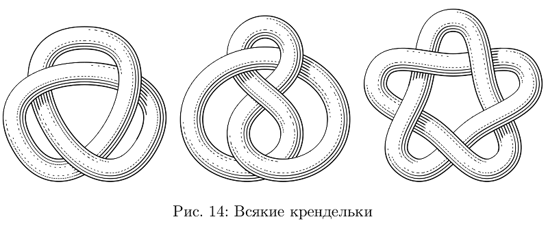
There is also a tool to tie the hoses in knots.
Shadows at nodes - some complication in the lighting model. In principle, no one bothers to use them in other cases, but I didn’t set myself the goal of going deep into the volume, so far this is not very convenient and does not work everywhere.
And, of course, we need a wood texture. The influence of the character of the growth of knots on the pattern of slices of growth rings is a topic for serious research. Very simplifying, you can imagine the one-year rings in parallel planes, which are distorted by knots. So, it is enough to describe the change of the plane by some not very tricky function (knot function) and consider a series of contour lines for the sum of a set of such functions as the desired pattern of year rings.
The eye from the picture above may slightly open, or squint, and the width of his pupil changes. There is no special meaning in this, but it turns out to be more vivid than if such trifles were mechanically the same everywhere.

Most often, the pictures were not very complex, but if you approach the matter seriously, many tasks need to be solved in order to illustrate them meaningfully. For example, Lopital’s block task (I don’t know how to call it correctly in Russian, it wasn’t in the textbook, just for an example): hanging on a rope of length l, suspended at point A, block, it is hooked to another rope suspended at the same height at point B, a load C is hanging on the second rope. It is asked if the ropes and the block are weightless, where will the load be? Surprisingly, the solution of the problem, and the construction are not so elementary, but, playing with several variables, you can easily make the picture exactly the one that would look best on the strip, while remaining true.
And what is the textbook? Alas, when almost all the illustrations and layout were ready, something happened there and it never came out. So, probably, some time later, I rewrote all the main pieces from the resulting library again and put the code on the github . Some Kunshtuki were not there: for example, electrical circuits or a function for drawing machines and tractors. Some - added: nodes, for example.
The whole kitchen does not work fast: it takes about a minute to collect all the pictures for this article from LuaLaTeX on my laptop with i5-4200U 1.6 GHz. For so many things, a pseudo-random number generator is used, so similar pictures will look slightly different not only inside one pass (this is a feature), but each next run will give pictures that are different from the previous one. But you can always set in the preamble
')
The most significant advantage of this solution is that each picture may be a small function of several variables; such a picture is easy, for example, to change in size and fit the stripes to specific unknown circumstances without disturbing important proportions, which is difficult to achieve with more traditional means. And still repeating elements - those balls and springs - can be made to behave much more interesting than the means of “human” vector editors allow.
I wanted to make pictures with shading, like the one found in old books.
To begin with, it was necessary to get lines of variable thickness. The main difficulty here is to build a curve that is more or less parallel to a given one and, as appropriate, changing the distance to a given one. I relied on the most probably primitive way in which the segments connecting the intermediate points of the Bezier curve are simply transferred in parallel to this distance. With the difference that this distance can vary along the curve.
In most cases, this allows for a tolerable result.
Sample code
Hereinafter, it is assumed that the library is downloaded and somewhere there is a line
or in LuaLaTeX:
input fiziko.mp; . The quickest way to start and see in ConTeXt (then beginfig and endfig not needed):\starttext
\startMPcode
input fiziko.mp;
\stopMPcode
\stoptext
or in LuaLaTeX:
\documentclass{article}
\usepackage{luamplib}
\begin{document}
\begin{mplibcode}
input fiziko.mp;

\end{mplibcode}
\end{document}
beginfig(3);
path p, q; % , , ,
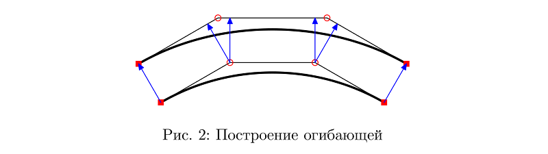
p := (0,-1/4cm){dir(30)}..(5cm, 0)..{dir(30)}(10cm, 1/4cm);
q := offsetPath(p)(1cm*sin(offsetPathLength*pi)); % — , — (offsetPathLength, 0 1), ,
draw p;
draw q dashed evenly;
endfig;
Now, from two such curves you can make a contour of the line of variable thickness.
Sample code
beginfig(4);
path p, q[];
p := (0,-1/4cm){dir(30)}..(5cm, 0)..{dir(30)}(10cm, 1/4cm);
q1 := offsetPath(p)(1/2pt*(sin(offsetPathLength*pi)**2)); %
q2 := offsetPath(p)(-1/2pt*(sin(offsetPathLength*pi)**2)); %
fill q1--reverse(q2)--cycle;
endfig;
The thickness should be limited to something below, otherwise too thin parts of the lines will be taken on by a raster when printing, and this is usually not very beautiful. One option is to make all the lines, the thickness of which is less than some value, with dashed lines of the same minimum thickness, such that the total amount of paint per unit length corresponds on average to that of the target thickness line. That is, instead of reducing the amount of paint from the sides of the line, begin to gnaw it with transverse stripes.
Sample code
beginfig(5);
path p;
p := (0,-1/4cm){dir(30)}..(5cm, 0)..{dir(30)}(10cm, 1/4cm);
draw brush(p)(1pt*(sin(offsetPathLength*pi)**2)); % , ,
endfig;
Now you can draw the balls. These may simply be concentric circles, the thickness of the lines which are determined by the function of the illumination of the ball at the points through which the lines pass.
Sample code
beginfig(6);
draw sphere.c(1.2cm);
draw sphere.c(2.4cm) shifted (2cm, 0);
endfig;
Another convenient primitive is “hoses”: roughly speaking, cylinders that can be bent in every direction. As long as they are of constant section, everything is simple with them.
Sample code
beginfig(7);
path p;
p := subpath (1,8) of fullcircle scaled 3cm;
draw tube.l(p)(1/2cm); % — ,
endfig;
If the thickness changes, it is necessary to change the number of strokes accordingly, while maintaining the average fill density unchanged, as well as to take into account changes in the thickness when calculating the illumination.
Sample code
beginfig(8);
path p;
p := pathSubdivide(fullcircle, 2) scaled 3cm;
draw tube.l(p)(1/2cm + 1/6cm*sin(offsetPathLength*10pi));
endfig;
There are more hoses with cross-hatching, but for them to solve the problem of preserving the average filling density turned out to be more difficult, so in many cases they still do not look very good.
Sample code
beginfig(9);
path p;
p := pathSubdivide(fullcircle, 2) scaled 3cm;
draw tube.t(p)(1/2cm + 1/6cm*sin(offsetPathLength*10pi));
endfig;
In principle, a lot of things can be made from hoses alone: from cones and cylinders to balusters.
Sample code
beginfig(10);
draw tube.l ((0, 0) -- (0, 3cm))((1-offsetPathLength)*1cm) shifted (-3cm, 0); %
path p;
p := (-1/2cm, 0) {dir(175)} .. {dir(5)} (-1/2cm, 1/8cm) {dir(120)} .. (-2/5cm, 1/3cm) .. (-1/2cm, 3/4cm) {dir(90)} .. {dir(90)}(-1/4cm, 9/4cm){dir(175)} .. {dir(5)}(-1/4cm, 9/4cm + 1/5cm){dir(90)} .. (-2/5cm, 3cm); %
p := pathSubdivide(p, 6);
draw p -- reverse(p xscaled -1) -- cycle;
tubeGenerateAlt(p, p xscaled -1, p rotated -90); % , tube.t, — — , — .
endfig;
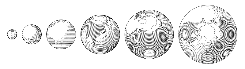
Something from what can be built from such parts is in the library. Let's say a globe is basically a ball.
Sample code
beginfig(11);
draw globe(1cm, -15, 0) shifted (-6/2cm, 0); % , ,
draw globe(3/2cm, -30.28367, 59.93809);
draw globe(4/3cm, -140, -30) shifted (10/3cm, 0);
endfig;
Although not: here the hatching goes along the parallels, and it is even more difficult to control the thickness of the stroke in order to preserve the filling density than in the case of cross-hatching on the hoses, so this is a separate type of ball.
Sample code
beginfig(12);
draw sphere.l(2cm, -60); %
draw sphere.l(3cm, 45) shifted (3cm, 0);
endfig;
A weight is an uncomplicated construction of two types of hoses of variable thickness.
Sample code
beginfig(13);
draw weight.s(1cm); %
draw weight.s(2cm) shifted (2cm, 0);
endfig;
There is also a tool to tie the hoses in knots.
Sample code not to clutter, only one node
beginfig(14);
path p;
p := (dir(90)*4/3cm) {dir(0)} .. tension 3/2 ..(dir(90 + 120)*4/3cm){dir(90 + 30)} .. tension 3/2 ..(dir(90 - 120)*4/3cm){dir(-90 - 30)} .. tension 3/2 .. cycle;
p := p scaled 6/5;
addStrandToKnot (primeOne) (p, 1/4cm, "l", "1, -1, 1"); % primeOne , p 1/4cm, "l" ( tube.l, tube.t ) «» "1, -1, 1" p
draw knotFromStrands (primeOne); % .
endfig;
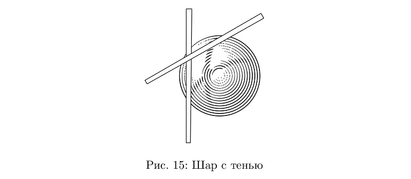
Shadows at nodes - some complication in the lighting model. In principle, no one bothers to use them in other cases, but I didn’t set myself the goal of going deep into the volume, so far this is not very convenient and does not work everywhere.
Sample code
beginfig(15);
path shadowPath[];
boolean shadowsEnabled;
numeric numberOfShadows;
shadowsEnabled := true; %
numberOfShadows := 1; %
shadowPath0 := (-1cm, -2cm) -- (-1cm, 2cm) -- (-1cm +1/6cm, 2cm) -- (-1cm + 1/8cm, -2cm) -- cycle; % , ,
shadowDepth0 := 4/3cm; % - «» ,
shadowPath1 := shadowPath0 rotated -60;
shadowDepth1 := 4/3cm;
draw sphere.c(2.4cm); % sphere.c tube.l
fill shadowPath0 withcolor white;
draw shadowPath0;
fill shadowPath1 withcolor white;
draw shadowPath1;
endfig;
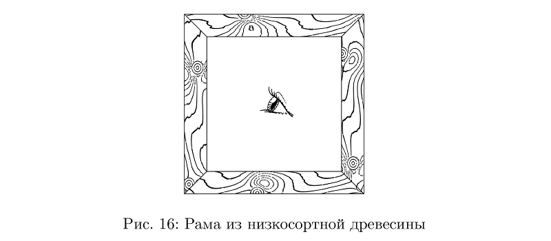
And, of course, we need a wood texture. The influence of the character of the growth of knots on the pattern of slices of growth rings is a topic for serious research. Very simplifying, you can imagine the one-year rings in parallel planes, which are distorted by knots. So, it is enough to describe the change of the plane by some not very tricky function (knot function) and consider a series of contour lines for the sum of a set of such functions as the desired pattern of year rings.
Sample code
beginfig(16);
numeric w, b;
pair A, B, C, D, A', B', C', D';
w := 4cm;
b := 1/2cm;
A := (0, 0);
A' := (b, b);
B := (0, w);
B' := (b, wb);
C := (w, w);
C' := (wb, wb);
D := (w, 0);
D' := (wb, b);
draw woodenThing(A--A'--B'--B--cycle, 0); % , A--A'--B'--B--cycle, 0
draw woodenThing(B--B'--C'--C--cycle, 90);
draw woodenThing(C--C'--D'--D--cycle, 0);
draw woodenThing(A--A'--D'--D--cycle, 90);
eyescale := 2/3cm; %
draw eye(150) shifted 1/2[A,C]; % 150
endfig;
The eye from the picture above may slightly open, or squint, and the width of his pupil changes. There is no special meaning in this, but it turns out to be more vivid than if such trifles were mechanically the same everywhere.
Sample code
beginfig(17);
eyescale := 2/3cm; % 1/2cm
draw eye(0) shifted (0cm, 0);
draw eye(0) shifted (1cm, 0);
draw eye(0) shifted (2cm, 0);
draw eye(0) shifted (3cm, 0);
draw eye(0) shifted (4cm, 0);
endfig;
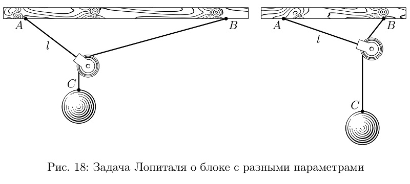
Most often, the pictures were not very complex, but if you approach the matter seriously, many tasks need to be solved in order to illustrate them meaningfully. For example, Lopital’s block task (I don’t know how to call it correctly in Russian, it wasn’t in the textbook, just for an example): hanging on a rope of length l, suspended at point A, block, it is hooked to another rope suspended at the same height at point B, a load C is hanging on the second rope. It is asked if the ropes and the block are weightless, where will the load be? Surprisingly, the solution of the problem, and the construction are not so elementary, but, playing with several variables, you can easily make the picture exactly the one that would look best on the strip, while remaining true.
Sample code
vardef lHopitalPulley (expr AB, l, m) = % AB l, m . ? : , , arithmetic overflow.
save A, B, C, D, E, o, a, x, y, d, w, h, support;
image(
pair A, B, C, D, E, o[];
path support;
numeric a, x[], y[], d[], w, h;
x1 := (l**2 + abs(l)*((sqrt(8)*AB)++l))/4AB; % ,
y1 := l+-+x1; %
y2 := m - ((AB-x1)++y1); %
A := (0, 0);
B := (AB*cm, 0);
D := (x1*cm, -y1*cm);
C := D shifted (0, -y2*cm);
d1 := 2/3cm; d2 := 1cm; d3 := 5/6d1; % ,
w := 2/3cm; h := 1/3cm; % . ,
o1 := (unitvector(CD) rotated 90 scaled 1/2d3);
o2 := (unitvector(DB) rotated 90 scaled 1/2d3);
E := whatever [D shifted o1, C shifted o1]
= whatever [D shifted o2, B shifted o2]; % ,
a := angle(AD);
support := A shifted (-w, 0) -- B shifted (w, 0) -- B shifted (w, h) -- A shifted (-w, h) -- cycle;
draw woodenThing(support, 0); % ,
draw pulley (d1, a - 90) shifted E; %
draw image(
draw A -- D -- B withpen thickpen;
draw D -- C withpen thickpen;
) maskedWith (pulleyOutline shifted E); %
draw sphere.c(d2) shifted C shifted (0, -1/2d2); %
dotlabel.llft(btex $A$ etex, A);
dotlabel.lrt(btex $B$ etex, B);
dotlabel.ulft(btex $C$ etex, C);
label.llft(btex $l$ etex, 1/2[A, D]);
)
enddef;
beginfig(18);
draw lHopitalPulley (6, 2, 11/2); % ,
draw lHopitalPulley (3, 5/2, 3) shifted (8cm, 0);
endfig;
And what is the textbook? Alas, when almost all the illustrations and layout were ready, something happened there and it never came out. So, probably, some time later, I rewrote all the main pieces from the resulting library again and put the code on the github . Some Kunshtuki were not there: for example, electrical circuits or a function for drawing machines and tractors. Some - added: nodes, for example.
The whole kitchen does not work fast: it takes about a minute to collect all the pictures for this article from LuaLaTeX on my laptop with i5-4200U 1.6 GHz. For so many things, a pseudo-random number generator is used, so similar pictures will look slightly different not only inside one pass (this is a feature), but each next run will give pictures that are different from the previous one. But you can always set in the preamble
randomseed := - , and all the same runs will produce the same pictures.Source: https://habr.com/ru/post/423571/
All Articles