Passed the mat, you can get married!

Introduction

The finite element method (FEM or FEM, they have abroad) has become firmly established in the practice of engineering calculations in the design of complex systems. To a large extent this concerns the strength calculations of mechanics. The application of this method, implemented by the appropriate software, significantly shortens the development cycle of the final device, making it possible to eliminate the mass of experimental checks required when using classical calculations based on the methods of reinforced metal and structural mechanics. To date, developed mass application software that implements the FEM. Powerful ANSYS is at the forefront, and CAD systems with an integrated FEM module (SolidWorks, Siemens NX, Creo Parametric, Compass 3D) are located at the sides of it and in an honorable distance.

CalculiX is strong, but difficult and incomprehensible. Fix that?


')
Naturally, the FEM has also penetrated into the field of education - in order to use it in real tasks, the training of relevant specialists is needed. In the capitals, in large technical universities, the situation in this area is more or less normal, and in our region the same ANSYS is used, for example, at the Department of Theory of Elasticity at the Southern Federal University. But on the periphery, in narrowly specialized and not rich universities, the situation is deplorable. And everything is simple - ANSYS costs about 2 million rubles for one workplace, and more than one place is required. Unfortunately, not all universities can afford to put 30-40 million on the organization of a computer class for learning how to apply FEM.

One alternative could be the use of free software in the learning process. Fortunately, such software is available. However, there are practically no Russian-language materials on its use. Correcting this situation, I am going to devote this article to the introduction to CalculiX - an open, free software package designed to solve linear and nonlinear three-dimensional problems of solid mechanics of a deformable body and fluid and gas mechanics using the finite element method.

1. What is CalculiX and where to get it. Installation in Windows

The CalculiX package is a set of console utilities that include a preprocessor for preparing initial data, an FEM solver, and a postprocessor for processing results. CalculiX is used both independently and as part of other products, among which the accelerating FreeCAD stands out. Another question is that CalculiX is still little known in our country, which is directly stated in the only article about it on this resource .

I will deliberately state the following material in relation to work in Windows OS, as the most common and used, including educational institutions. In this case, the use of many free programs in it is a frank pain.

If you take the package for Windows from the official site CalculiX, then it becomes completely incomprehensible what to do with it further. In conjunction with the English-language documentation, it puts a cross on this product for many, and then results in poisonous comments about the impossibility of using it. And partly this is true - the threshold of entry is really high. But still we will try.

There are a number of informal relatively newbie-friendly builds of this miracle for Windows, among them bConverged CalculiX for Windows . We swing the distribution kit from here , we unpack, and we establish it by a standard method "further, further ...". Installation, therefore, does not constitute a special sacrament and is quite accessible to the inexperienced user. The main working environment in this package uses the text editor SciTE, which integrates calls to the components of CalculiX, as well as the possibility of interactive command entry and it looks like this (clickable).

2. The problem of the bending of a beam and its analytical solution using the strength of materials method

Take a simple student's task - the bending of a steel beam, one end of which is clamped, and the vertical force F is applied to the other.



The parameters of the problem are as follows: F = 10 kN; l = 1 m - the length of the beam; h = 0.1 m and b = 0.05 m are the dimensions of the cross section. For simplicity, we will not take into account the own weight of the beam, since it, with a beam mass of 39 kg, is significantly less than the applied load. Find the maximum normal stress in the cross section of the beam as well as calculate the deflection of the beam due to the bending deformation.

Any student who did not skip mat will easily solve such a problem. In order not to embarrass the noble dons, I will wrap all the details of the decision in a spoiler


For those who are too lazy to look under the spoiler, immediately give the answer to the problem: the maximum normal stress in the beam section $$$\ sigma_x = 119$ MPa, and the maximum deflection is 3.97 millimeters. These figures are given for later comparison with what the procedure for solving this problem in CalculiX will give us.

3. Preparation of geometry and computational grid

First of all, it is necessary to enter into CalculiX geometrical data about the part in question. Yes, it is possible to export geometry from CADs, as is done in the same ANSYS, but we will go through the torment and enter the geometry manually. Open the SciTE editor from the bConverged bundle and type the following text there

pnt p1 0 0 0
pnt p2 0.25 0 0
pnt p3 0.5 0 0
pnt p4 0.75 0 0
pnt p5 1.0 0 0

Save the file with the name beam.fbd and press F10 to start the preprocessing. We will see something like the following.



The pnt command creates a point in space with given coordinates and its syntax is

pnt [ ] [x] [y] [z]

Now connect these points with lines by adding the following text to the file

line l1 p1 p2 25
line l2 p2 p3 25
line l3 p3 p4 25
line l4 p4 p5 25

getting after pressing F10 the following picture



Team

line [ ] [ 1] [ 2] [ ]

creates a line connecting the points indicated in it, adding intermediate points dividing the line into a specified number of segments (in our case, 25 for each line). This is useful later for generating the grid. Now do the feint ears

seta lines l l1 l2 l3 l4
swep lines sweeplines tra 0 0 0.1 10

First team

seta [ ] [ 1] ... [ N]

combines several objects into a set with the specified name. In essence, this is an analogue of grouping objects. Next team

swep [ ] [ ] [ ] [, ] []

moves the selected set of objects to form a new set. Relocatable objects are copied. In this case, the movement of points forms lines, the movement of lines — the surface, the movement of surfaces — is solid volumes. In our case, we shift the set of lines of lines along the Z axis by 0.1 meters, while the lines that form are divided into 10 segments. Hit F10 ... uh, what is it?



GHM, blank screen ... It fixes easily, just add lines to the end of the script.

plot pa all
plus la all

These commands indicate to draw all points (pa) and add all lines (la) to the display, after which we get the result



Now create surfaces based on the set of lines we created.

seta surfaces s A001 A002 A003 A004

adding the display of these surfaces at the very end of the script

plus sa all




Now we will perform another shift, now along the Y axis by 0.05 meters, developing all the lines that are formed when the line is displaced by 5 segments.

swep surfaces swepsurface tra 0.0 0.05 0.0 5

We get something in the spirit



The resulting image can be rotated by holding down the left mouse button and removing the display of points and lines, we will see something intelligible



Yeah ... CalculiX is far from the visual concepts familiar to the mainstream user, but nevertheless we built the geometry of our beam.

Geometry, geometry, but to generate the grid, we will make the next move - remove all the plot and plus commands and wrap the geometry generation code in the seto and setc commands, like this

seto beam
pnt p1 0 0 0
pnt p2 0.25 0 0
pnt p3 0.5 0 0
pnt p4 0.75 0 0
pnt p5 1.0 0 0
line l1 p1 p2 25
line l2 p2 p3 25
line l3 p3 p4 25
line l4 p4 p5 25
seta lines l l1 l2 l3 l4
swep lines sweeplines tra 0 0 0.1 10
seta surfaces s A001 A002 A003 A004
swep surfaces swepsurface tra 0 0.05 0 5
setc beam

This pair of commands combines all the created geometry into a certain geometry block named beam. Now this geometric group can be skipped through the generation of the grid, specifying after all the above command code

elty beam he8
mesh beam

- generates a grid consisting of parallelepipeds (he8) based on a geometry with the name beam. Now output the generated mesh to a file.

send beam abq

- output of the grid to a file named beam.msh in the format of the FEM-package ABAQUS (there is such a proprietary package of FEM calculations and CalculiX understands its format)



Thus, the grid is generated, you can look into the file beam.msh and see something like this there

*NODE, NSET=Nbeam
1,0.000000000000e+000,0.000000000000e+000,1.000000000000e-001
2,0.000000000000e+000,0.000000000000e+000,9.000000000000e-002
3,0.000000000000e+000,1.000000000000e-002,9.000000000000e-002
4,0.000000000000e+000,1.000000000000e-002,1.000000000000e-001
5,1.000000000000e-002,0.000000000000e+000,1.000000000000e-001
6,1.000000000000e-002,0.000000000000e+000,9.000000000000e-002
7,1.000000000000e-002,1.000000000000e-002,9.000000000000e-002
8,1.000000000000e-002,1.000000000000e-002,1.000000000000e-001
9,0.000000000000e+000,2.000000000000e-002,9.000000000000e-002
10,0.000000000000e+000,2.000000000000e-002,1.000000000000e-001
11,1.000000000000e-002,2.000000000000e-002,9.000000000000e-002
.
.
.
.
*ELEMENT, TYPE=C3D8, ELSET=Ebeam
1, 1, 2, 3, 4, 5, 6, 7, 8
2, 4, 3, 9, 10, 8, 7, 11, 12
3, 10, 9, 13, 14, 12, 11, 15, 16
4, 14, 13, 17, 18, 16, 15, 19, 20
5, 18, 17, 21, 22, 20, 19, 23, 24
6, 5, 6, 7, 8, 25, 26, 27, 28
7, 8, 7, 11, 12, 28, 27, 29, 30
8, 12, 11, 15, 16, 30, 29, 31, 32
9, 16, 15, 19, 20, 32, 31, 33, 34

Apparently, this is a list of vertices of mesh elements with their coordinates, followed by a list of faces. To make this whole thing look more beautiful, let's use the interactive mode CalculiX. To do this, leaving the graphical window active , enter the following commands in sequence

plot f beam

- display all faces of the geometry

view edge off

- disable edges display

view elem

- enable the display of grid elements. Entering each command is completed by pressing Enter, the entered commands are displayed in the SciTE window at the bottom right, like this



Yes, it is impossible to call this super-convenient, but nevertheless we will get an image of the generated mesh.



I note that all the intermediate points that were created during the creation of the geometry have become grid nodes. Thus, we obtained a hexagonal grid with a size of 100 x 10 x 5 knots, with an edge size of 10 mm. The file beam.fbd we created describes the geometry of the problem and the process of creating a grid.

4. Setting restrictions

An important step in the application of FEM is the specification of restrictions on the movement of points of the structure, that is, the consideration of the connections imposed on it. In our case, one of the ends of the beam is clamped, and therefore we can assume that one of its ends is completely motionless. We need to tell the solver which FE nodes are fixed. We press F10 with the open file beam.fbd, we wait for the appearance of a window with the image of a beam



In interactive mode, enter commands
rot -y
plot n beam

The first command expands the model so that the Y axis looks away from us, the second one includes drawing nodes (n) of the QE grid. Moving the model (holding the right mouse button) and scaling the image (holding the mouse wheel) we achieve such a picture



Now you need to select all the nodes that we want to define as fixed. For this, we again use the interactive data entry mode. Recruit team

qadd fixed

that starts creating a node set named fixed. The cursor on the graphics window switches to the selection of items - displayed as an arrow with a small square. Put the cursor like this



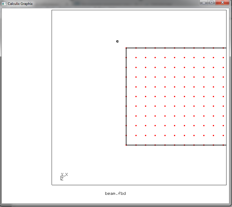
and press the r key. And then put the cursor like this



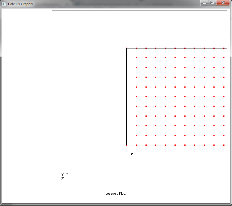
and press r again. Thus, we have formed a rectangular selection area, the diagonal of which is given by the cursor positions marked by pressing r. Select this rectangle we need nodes lying on the end of the beam



click a and then click n, highlighting the marked nodes. In the console window there will be a footcloth with a list of selected nodes (the image is clickable)



Enter q to exit the selection mode and the command

plus n fixed g

to display the fixed group nodes in green (g). Now we can see which nodes we will have in the pinning condition



Now we have to unload these nodes as a constraint file, which is then fed to the input of the solver. To do this, type the command

send fixed abq spc 123

- unload a group of fixed nodes as a file of restrictions in the ABAQUS (abq) format, limiting the movement of all nodes of the group along all three degrees of freedom (1 - X axis, 2 - Y axis, 3 - Z axis). As a result, the file is fixed_123.bou, as follows

** BOUNDARY based on fixed
1, 1, ,
2, 1, ,
3, 1, ,
4, 1, ,
9, 1, ,
10, 1, ,
13, 1, ,
14, 1, ,
17, 1, ,
.
.
.


- in fact, this is a list of all nodes and the number of degrees of freedom, which is limited to the movement of this node.

5. Task loads

After we secured our beam, we will try to load it. Turn on the face and element display mode again.

plot f beam
view edge off
view elem

Orient the image so that we can see the upper part of the loose end of the beam.



Let's switch to object selection mode.

qadd load

Move the cursor to the desired edge and press f



The face is highlighted in purple, and a description appears in the console window so that it is added to the load set.

qadd load
2541 e:3873 s:6 n= 5298 5310 5312 5300

Press a to end the formation of the set, press q to exit the selection mode. Apply pressure to the selected face, giving a resultant force of 10,000 N. It is easy to calculate that the area of ​​the selected face is 1 cm ² , which means that the pressure required is 10 ⁸ Pa. We set this load with the command

send load abq pres 1e8

- displays the load in the file load.dlo in ABAQUS format. File looks like this

** Pressure based on load
3873, P6, 100000000.000000

The number of the grid element, its face and the amount of pressure on this face is indicated. Thus, the preparation of the source data can be considered complete.

6. Description of input data and launch solver

All those data — grid, constraints, and loads — should now be thrown to the input of the FEM solver, for which we form an input file of this type

beam.inp
*HEADING
Model: CalculiX Beam Input File for Habrahabr article
*INCLUDE,INPUT=beam.msh
*BOUNDARY
*INCLUDE,INPUT=fixed_123.bou
*MATERIAL,NAME=EL
*ELASTIC
2e11,0.3
*SOLID SECTION,ELSET=Ebeam,MATERIAL=EL
*STEP
*STATIC
*DLOAD
*INCLUDE,INPUT=load.dlo
*NODE FILE
U
*EL FILE
S
*END STEP


Let me explain in more detail what is what. The first section of the file

*HEADING
Model: CalculiX Beam Input File for Habrahabr article
*INCLUDE,INPUT=beam.msh

sets the description of the task and includes the file with the CE mesh beam.msh. The next section forms the boundary conditions - those connections that we defined in the file fixed_123.bou

*BOUNDARY
*INCLUDE,INPUT=fixed_123.bou


We should not forget about the material that we define elastic, determining its Young modulus and Poisson’s ratio. Values ​​take average values ​​for structural steel.

*MATERIAL,NAME=EL
*ELASTIC
2e11,0.3
*SOLID SECTION,ELSET=Ebeam,MATERIAL=EL

The last section sets the type of task - the calculation of static loading and those loads, from the file load.dlo, which act

*STEP
*STATIC
*DLOAD
*INCLUDE,INPUT=load.dlo
*NODE FILE
U
*EL FILE
S
*END STEP


Having checked that we have in SciTE an open tab with the file beam.inp we press Ctrl + F10, thus launching the solver. We get the exhaust, telling us that CalculiX counted something for us. Vyhlob, so as not to clutter the text I quote under the spoiler

7. Postprocessing and decision analysis

The results obtained by the solver require processing by the postprocessor. To call it, press Shift + F10 and get the graphic window with the image of the beam. Click on the left side of this window, beyond the frame with the image of the beam and get the menu



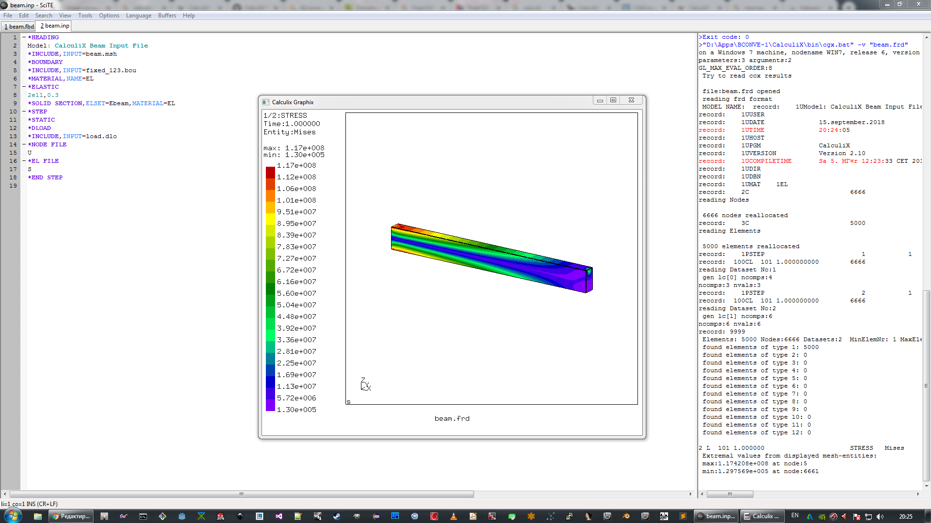
What interests us? Stresses in the beam sections - choose Datasets -> STRESS. The menu will disappear, but we call it again and select Datasets -> Entities -> Mises. As a result, the von Mises equivalent voltage display mode is turned on.



So - the moment of truth! The maximum equivalent stress in the cross section of the beam is 117 MPa, which slightly differs from the result of the reinforcement. But! Solving the problem of resistance to mathematics, we did not take into account the shear stresses in bending and shear, and we considered only the normal bending stresses. What will happen to the deflection? Go to the menu: Datasets -> DISP and Datasets -> Entities -> D3



We observe that the maximum displacement corresponds to the loaded end of the beam and is equal to 3.96 millimeters! Excellent and correlated with our calculation using the Mohr integral.

By simple manipulations, which can be read here , the beam deformations are also generated.

Draw conclusions

"Uh-uh, man, wait, what's next ?!" Hmmm, dude can't fit in one article all the variety of questions that are raised at the mention of FEM in general, and CalculiX in particular. The article and so left a voluminous and rather boring. And its purpose is to explain two things in intelligible language:

1. Open Source did not pass by software for FEM analysis
2. Studying and using this software is not as difficult as it may seem at first glance.

Enough for a review article? I think yes. In preparing the article, the following sources were used:

1. Calculix FEA Beam - was the basis of all the material presented. Since here the experience gained by the author is added and all the code written by him in the process of writing the article is not a translation, but a tutorial in Russian
2. Official CalculiX Manual

Sample code is available on Gitlab .

In conclusion, I note - I am not strong, I did not have the maturity at the university. A little later, life (and love!) Forced me to know its very foundations. So blunders, perhaps, are present in the text, about which I wait for malicious comments and give a promise to take into account all the comments.

Thank you for attention!