You have not finished saying the word “hello”, and we already know who you are
This can be done by our neural network, which recognizes a person by one uttered syllable. However, the topic of this article does not deal directly with voice identification, although it will be associated with it. We will talk about neural network features, the so-called d-vector, which can be used in sound processing tasks: from verification to recognition of speech and emotions.
Depending on the sampling frequency, there can be from 8 to 48 thousand numbers in one second of sound. They can be represented as deviations from the equilibrium position of the membrane speaker or microphone. In fact, such a sound description is redundant: the amplitude of the signal at the next time instant strongly depends on the previous one, which hints that this signal can be effectively compressed without much loss of information. There are a huge number of ways to reduce the dimension of the signal, and most of them are based on the physical properties of sound and the features of human hearing.

Mem 1.
')
Before neural networks have proven themselves (in a broad sense), the community has worked with so-called hand-crafted tags. The most famous and widely used of them is Pitch and MFCC . The first has the physical meaning of the frequency of oscillations of the vocal cords, which differ, for example, for different people, and also depend on intonation. The idea of chalk-cepstral coefficients (MFCC) is based on the nonlinearity of human perception of sound, namely, frequency and volume. It seems to a person that one sound is higher by some other than another, if in reality their frequencies differ a certain number of times.
These and other manually calculated signs are irreversible in the sense that some part of the signal is lost irretrievably. In some tasks this is not critical, but I would like to come up with a more universal and working approach.
The key to solving this problem is the Fourier transform. With it, you can imagine the sound signal as the sum of waves with different frequencies and amplitudes. In fact, speech is not stationary in the sense that its spectrum will be qualitatively different at different points in time. This allows us to consider it in the time-frequency representation, using spectrograms .
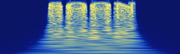
To build a spectrogram, you need to split the sound into overlapping frames with a length of several tens of milliseconds. For each of them, calculate the Fourier transform and write their modules into columns in the spectrograms. Moreover, such a transformation is almost reciprocal, that is, using the inverse Fourier transform and the Griffin-Lima algorithm, you can restore the original audio signal (in fact, there is a loss of information, because the Fourier transform is generally complex, and the spectrogram is real-valued, and to approximately reconstruct the phases, the iterative Griffin-Lima algorithm is usually used. So, if you take the logarithm of the amplitudes, you get these images:

Spectrogram 5 seconds of speech.
And it is convenient to process them with convolutional networks.
Such tasks are often used in image processing tasks: there are large databases with examples of different objects (for example, ImageNet). You can train a large grid to recognize them, and then further train it on our specific task, or take the output from one of the inner fully connected layers. It is believed that such an architecture will calculate good informative features for the input images. Experience suggests that the results will almost always be better than if we trained the neural network from scratch.
The idea of d-vectors (generally d-vectors, but sometimes they are called x-vectors) is similar to the use of pre-trained grids on ImageNet, except for the fact that there are no similar bases for spectrograms. Autoencoders can be considered as a possible way out of the situation, but a priori they do not know what to look for in the spectrogram, therefore, they do not work satisfactorily.
Attention, the main part of this article begins.
The task of verifying a person by voice is widely known, where you need to determine by the input speech segment which of the people in the database said it. In fact, the construction of such systems is a separate science, and there are many different add-ons (speech duration; does everyone need to speak the same text; staging one vs one or one vs all), which are critical under different conditions, but we need to pay attention to something else.
Namely: how high-quality features will be if we pre-train the grid to recognize a person. Everything is done for the sake of signs.
This will help us intuition and article 2015. In it, the authors teach the grid to recognize a person by face (face recognition). The trick of this work is to use Triplet Loss.
His idea is very simple: we normalize features from the penultimate layer so that they lie on the unit sphere, and demand that the points from one class lie close, and from different ones - far away. This can be achieved as follows: for each teaching example (anchor) we find in the sample two more from the same and from another class - positive and negative. Then for these triples of points we form a loss:
\ begin {equation}
\ Big [\ Vert f (x ^ a) - f (x ^ p) \ Vert - \ Vert f (x ^ a) - f (x ^ n) \ Vert + \ alpha \ Big] _ +,
\ end {equation}
where x is the input picture, f is the output of the grid after normalization, alpha is the manually selectable parameter, [] _ {+} is the ReLU function. Qualitatively, the value of this loss is zero, if the distance between the anchor and positive points is greater than the distance between anchor and negative at least by alpha, and the greater, the smaller the difference between two different classes.

Illustration of what happens with features after training with Triplet Loss.
By the way, it is possible to form triples rationally. At some point, the value of the loss will be small, and to speed up learning, you can look for negative examples not among all the other classes, but consider only those close to anchor. But for large data sets it is difficult, because you need to consider pairwise distances between classes, which change after each iteration of network training.
Triplet Loss has an advantage over the Categorical Crossentropy, which is used in the usual classification. A model trained with cross-entropy will try to shove all the points of one class into an area that is increasingly smaller in volume, and information that is unnecessary for a specific task can be lost. And we do not want this, because we are going to use the neural network as a feature generator, and not for verification. Triplet Loss has this property to a much lesser extent: it is more important for him to spread the different classes to different areas on a single sphere than to miss one class.

Mem 2.
The last thing to do before learning the feature generator on spectrograms is to determine their size. Obviously, the accuracy of the classification will be the higher, the longer the period of time we will consider, but the more “average” the signs will be. Therefore, it is reasonable to use such a signal length so that 1-3 phonemes (syllables) fall into it - half a second seems appropriate.
For training, we take VoxCeleb2 datasets, where each of the 6300 speakers has several separate audio recordings of several minutes each (made in different conditions). We use part of the audio files for training, and the rest - for validation, we choose the convolution network architecture, add Triplet Loss to it and learn.
The results were very cool. For almost 2 weeks of training at 1080Ti (yes, for so long), the classification accuracy reached 55%. It would seem, not very much, but the accuracy of top-5 is 78%, and if we consider only the loudest half of the fragments, and these are mainly shock vowels, then the accuracy of top-5 will increase to 91%. We can say that we are able to identify a person by one phrase with decent accuracy. But it is not important.
Mem 3.
After all, everything was started for features that can be obtained as an exit from the penultimate one before the classification of the neural network layer. We checked them on our tasks, and everywhere the results were obtained better than when using classical approaches to calculate signs. For example, in the task of recognizing emotions, the use of d-vectors allowed us to bypass state-of-the-art by 4%, and the corresponding article was accepted at the FICC 2019 conference. However, the recognition of emotions is a completely different story, which we will describe later.
Author: Gregory Sterling sterling239 , deep learning expert, Neurodata Lab.
Materiel
Depending on the sampling frequency, there can be from 8 to 48 thousand numbers in one second of sound. They can be represented as deviations from the equilibrium position of the membrane speaker or microphone. In fact, such a sound description is redundant: the amplitude of the signal at the next time instant strongly depends on the previous one, which hints that this signal can be effectively compressed without much loss of information. There are a huge number of ways to reduce the dimension of the signal, and most of them are based on the physical properties of sound and the features of human hearing.
Mem 1.
')
Before neural networks have proven themselves (in a broad sense), the community has worked with so-called hand-crafted tags. The most famous and widely used of them is Pitch and MFCC . The first has the physical meaning of the frequency of oscillations of the vocal cords, which differ, for example, for different people, and also depend on intonation. The idea of chalk-cepstral coefficients (MFCC) is based on the nonlinearity of human perception of sound, namely, frequency and volume. It seems to a person that one sound is higher by some other than another, if in reality their frequencies differ a certain number of times.
These and other manually calculated signs are irreversible in the sense that some part of the signal is lost irretrievably. In some tasks this is not critical, but I would like to come up with a more universal and working approach.
The key to solving this problem is the Fourier transform. With it, you can imagine the sound signal as the sum of waves with different frequencies and amplitudes. In fact, speech is not stationary in the sense that its spectrum will be qualitatively different at different points in time. This allows us to consider it in the time-frequency representation, using spectrograms .
To build a spectrogram, you need to split the sound into overlapping frames with a length of several tens of milliseconds. For each of them, calculate the Fourier transform and write their modules into columns in the spectrograms. Moreover, such a transformation is almost reciprocal, that is, using the inverse Fourier transform and the Griffin-Lima algorithm, you can restore the original audio signal (in fact, there is a loss of information, because the Fourier transform is generally complex, and the spectrogram is real-valued, and to approximately reconstruct the phases, the iterative Griffin-Lima algorithm is usually used. So, if you take the logarithm of the amplitudes, you get these images:
Spectrogram 5 seconds of speech.
And it is convenient to process them with convolutional networks.
Such tasks are often used in image processing tasks: there are large databases with examples of different objects (for example, ImageNet). You can train a large grid to recognize them, and then further train it on our specific task, or take the output from one of the inner fully connected layers. It is believed that such an architecture will calculate good informative features for the input images. Experience suggests that the results will almost always be better than if we trained the neural network from scratch.
The idea of d-vectors (generally d-vectors, but sometimes they are called x-vectors) is similar to the use of pre-trained grids on ImageNet, except for the fact that there are no similar bases for spectrograms. Autoencoders can be considered as a possible way out of the situation, but a priori they do not know what to look for in the spectrogram, therefore, they do not work satisfactorily.
We need to go deeper
Attention, the main part of this article begins.
The task of verifying a person by voice is widely known, where you need to determine by the input speech segment which of the people in the database said it. In fact, the construction of such systems is a separate science, and there are many different add-ons (speech duration; does everyone need to speak the same text; staging one vs one or one vs all), which are critical under different conditions, but we need to pay attention to something else.
Namely: how high-quality features will be if we pre-train the grid to recognize a person. Everything is done for the sake of signs.
This will help us intuition and article 2015. In it, the authors teach the grid to recognize a person by face (face recognition). The trick of this work is to use Triplet Loss.
His idea is very simple: we normalize features from the penultimate layer so that they lie on the unit sphere, and demand that the points from one class lie close, and from different ones - far away. This can be achieved as follows: for each teaching example (anchor) we find in the sample two more from the same and from another class - positive and negative. Then for these triples of points we form a loss:
\ begin {equation}
\ Big [\ Vert f (x ^ a) - f (x ^ p) \ Vert - \ Vert f (x ^ a) - f (x ^ n) \ Vert + \ alpha \ Big] _ +,
\ end {equation}
where x is the input picture, f is the output of the grid after normalization, alpha is the manually selectable parameter, [] _ {+} is the ReLU function. Qualitatively, the value of this loss is zero, if the distance between the anchor and positive points is greater than the distance between anchor and negative at least by alpha, and the greater, the smaller the difference between two different classes.
Illustration of what happens with features after training with Triplet Loss.
By the way, it is possible to form triples rationally. At some point, the value of the loss will be small, and to speed up learning, you can look for negative examples not among all the other classes, but consider only those close to anchor. But for large data sets it is difficult, because you need to consider pairwise distances between classes, which change after each iteration of network training.
Triplet Loss has an advantage over the Categorical Crossentropy, which is used in the usual classification. A model trained with cross-entropy will try to shove all the points of one class into an area that is increasingly smaller in volume, and information that is unnecessary for a specific task can be lost. And we do not want this, because we are going to use the neural network as a feature generator, and not for verification. Triplet Loss has this property to a much lesser extent: it is more important for him to spread the different classes to different areas on a single sphere than to miss one class.
Mem 2.
The last thing to do before learning the feature generator on spectrograms is to determine their size. Obviously, the accuracy of the classification will be the higher, the longer the period of time we will consider, but the more “average” the signs will be. Therefore, it is reasonable to use such a signal length so that 1-3 phonemes (syllables) fall into it - half a second seems appropriate.
For training, we take VoxCeleb2 datasets, where each of the 6300 speakers has several separate audio recordings of several minutes each (made in different conditions). We use part of the audio files for training, and the rest - for validation, we choose the convolution network architecture, add Triplet Loss to it and learn.
The results were very cool. For almost 2 weeks of training at 1080Ti (yes, for so long), the classification accuracy reached 55%. It would seem, not very much, but the accuracy of top-5 is 78%, and if we consider only the loudest half of the fragments, and these are mainly shock vowels, then the accuracy of top-5 will increase to 91%. We can say that we are able to identify a person by one phrase with decent accuracy. But it is not important.
Mem 3.
After all, everything was started for features that can be obtained as an exit from the penultimate one before the classification of the neural network layer. We checked them on our tasks, and everywhere the results were obtained better than when using classical approaches to calculate signs. For example, in the task of recognizing emotions, the use of d-vectors allowed us to bypass state-of-the-art by 4%, and the corresponding article was accepted at the FICC 2019 conference. However, the recognition of emotions is a completely different story, which we will describe later.
Author: Gregory Sterling sterling239 , deep learning expert, Neurodata Lab.
Source: https://habr.com/ru/post/422635/
All Articles