Hide without hiding. Once again about LSB-steganography, chi-square and ... singularity?

Today, we will again fly the old nest and talk about how to hide a bunch of bits in a picture with a cat, look at several available tools and analyze the most popular attacks. And it would seem, what have the singularity?

As they say, if you want to understand something, then write about this article on Habr! (Beware, a lot of text and pictures)



Steganography (literally from the Greek "secret writing") is the science of transferring hidden data (stego messages) in other open data (stegocontainers) while hiding the very fact of data transfer. Do not worry, in fact, everything is not so difficult.
')
So, where in the image can you hide the message without anyone noticing?

And there are only two places: metadata and the image itself. The latter is quite simple, just type in “exif” in Google. So let's start immediately with the second.

Least Significant Bit

The most popular color model is RGB, where the color is represented as three components: red, green and blue . Each component is encoded in the classic version using 8 bits, that is, it can take a value from 0
to 255. It is here that the least significant bit is hidden. It is important to understand that there are as many as three such bits per RGB color.

To present them more clearly, we will do a couple of small manipulations.

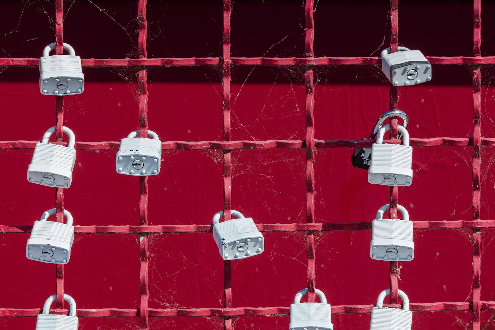
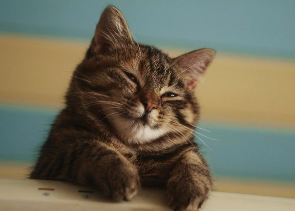
As promised, take a picture with a cat in png format.



We divide it into three channels and in each channel we take the least significant bit. Create three new images, where each pixel denotes a NSB. Zero - pixel white, unit respectively black.

We get this.




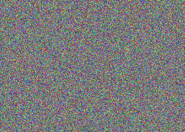
But, as a rule, the image is found in the "assembled". To represent the three components of the NSB in one image, it is enough to replace the component in the pixel, where the NSB is equal to one, replace with 255, and in the opposite case replace it with 0.

But no less significant.

Imagine that everything we saw in the last picture is ours and we have the right to do anything we want with it. Then we take it as a stream of bits, where we can read from and where we can write to.

We take the data that we want to intersperse into the image, present them in the form of bits and write down in place of the already existing ones.

To extract this data, read the NSB as a bitstream and bring it to the desired form. To find out how many bits are to be counted, as a rule, the size of the message is recorded at the beginning. But this is the implementation details.

It should be noted that in about 50% of cases, the bits that we want to record, and the bits in the picture will be the same and we will not have to change anything.

That's all, this method ends.

Why does this work?

Look at the pictures below.

This is an empty stegcontainer:



This is 95% full:



See the difference? And she is. Why is that?

Let's look at two colors: (0, 0, 0) and (1, 1, 1), that is, the colors that are different only in the NCB in each component.



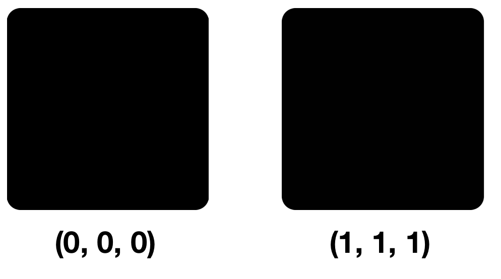
Small differences in pixels in the first, second and third views will not be noticeable. The fact is that our eye can distinguish about 10 million colors, and the brain is only about 150. The RGB model also contains 16,777,216 colors. Try to distinguish them all here.

From command line

There are not many publicly available command line tools that represent LSB steganography.

The most popular can be found in the table below.

Tulsa	File types	Description	Concealment	Extract
openstego	PNG	Can be used not just for hiding data, but also for water marks. Uses RandomLSB - improved write LSB algorithm in Random Least Significant Bit. Supports encryption. It also has a GUI.	openstego embed -mf secret.txt -cf cover.png -p password -sf stego.png	openstego extract -sf openstego.png -p abcd -xf output.txt
stegano	PNG	Works not only with classic LSB. It has flexible setting. Can used as Python module. Most attractive (as for me).	stegano-lsb hide - input cover.jpg -f secret.txt -e UTF-8 - output stego.png	stegano-lsb reveal -i stego.png -e UTF-8 -o output.txt
cloackedpixel	PNG, JPG	Simple tulza. Copes poorly with great message. (More precisely, nothing at all) Supports encryption.	cloackedpixel hide cover.jpg secret.txt password	cloackedpixel extract cover.jpg-stego.png output.txt password
LSBSteg	PNG, BMP	Small program on Python with readable code.	LSBSteg encode -i cover.png -o stego.png -f secret.txt	LSBSteg decode -i stego.png -o output.txt

Where's the cat?

And the first in the list of attacks on LSB steganography is a visual attack. It sounds strange, doesn’t it? After all, the cat with a secret did not present itself as a filled stegocontainer at first glance. Hmmm ... You just need to know where to look. It is easy to guess that only the NSB deserve our close attention.

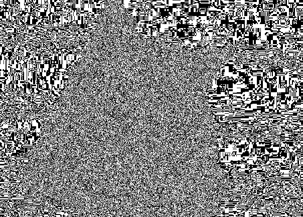
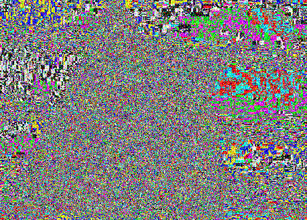
In the filled stegcontainer, the image from the NCB looks like this:



Do not believe? Here is the NCB from all three channels separately:




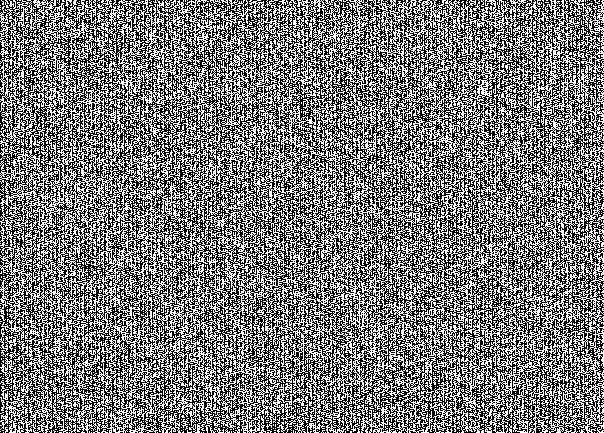
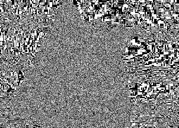
This is specific for hiding the message “picture” in the NZB. At first glance, this seems like a simple noise. But by consideration the structure is looked through. Here you can see that the stegcontainer is filled to capacity. If we took the message to 30% of the capacity of the poor cat, we would get the following picture:


His NCB:



~ 70% of the cat remained unchanged.

There is to make a small digression and talk about the size. What is 30% cat? The size of the cat is 603x433 pixels. 30% of this size is equal 78459 pixels. Each pixel contains 3 bits of information. A total of 78459 3 = 235377 bits or slightly less than 30 kilobytes fit into 30% of the seal. And in the whole cat fit about 100 kilobytes. So it goes.

But we are here for a reason. How can you fool your eyes?
My first thought: put a message in the noise. But it was not there. Next, a fragment of the filled stegocontainer and its LSB.



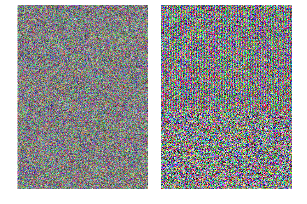
By applying a little effort, we can still distinguish the familiar structure. Do not lose hope, gentlemen!

Hee hee hee

A lot of things break statistics, you know.

Changing something in the picture, we change its statistical properties. It is enough for analytics to find a way to fix these changes.

Andreas Vesfield and Andreas Pfitzmann from the University of Dresden began to use the good old chi-square for this in their work “Attacks on Steganographic Systems”, which can be found here.

Hereinafter we will talk about attacks within the same color plane, or in the context of RGB, about attacks on one channel. The results of each attack can lead to an average and get the result for the "collected" image.

So, the Chi-square attack is based on the assumption that the probability of simultaneous appearance of neighboring (different for the least significant bit) colors (pair of values) in an unfilled stegocontainer is extremely small. This is true, you can believe it. In other words, the number of pixels of two adjacent colors is significantly different for an empty container. All we need to do is count the number of pixels of each color and apply a couple of formulas. In fact, this is a simple task to test the hypothesis using the chi-square test.

A bit of math?

Let h be an array in the i-th place containing the number of pixels of the i-th color in the image under study.

Then:

1. Measured color frequency $$$i = 2k$ :
   

   $$

   $$n_k = h [2k], ~ k \ in [0, 127];$$
   
   
2. Theoretically Expected Color Frequency $$$i = 2k$ :
   

   $$

   $$n_k ^ * = \ frac {h [2k] + h [2k + 1]} {2}, ~ k \ in [0.127];$$
   
   

Translating this into Python will result in something like this:

for k in range(0, len(histogram) // 2): expected.append(((histogram[2 * k] + histogram[2 * k + 1]) / 2)) observed.append(histogram[2 * k]) 

Where histogram is the number of pixels of color i in the image, $$$i \ in [0, 255]$

The chi-square criterion for the number of degrees of freedom k-1 is calculated as follows (k is the number of different colors, that is 256):

$$

$$\ chi_ {k-1} ^ 2 = \ sum_ {i = 1} ^ {k} \ frac {(n_k - n_k ^ *) ^ 2} {n_k ^ *};$$

And finally, P is the probability that the distribution $$$n_i$ and $$$n_i ^ *$ under these conditions are equal (the probability that we have a filled stegocontainer). It is calculated by integrating the smoothness function:

$$

$$P = 1 - \ frac {1} {2 ^ {\ frac {k-1} {2}} \ Gamma (\ frac {k-1} {2})} \ int_0 ^ {\ chi_ {k-1 } ^ 2} e ^ {- \ frac {x} {2}} x ^ {\ frac {k-1} {2} -1} dx;$$

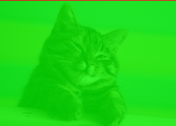
It is most effective to apply chi-square not to the whole image, but only to its parts, for example, to lines. If the calculated probability for the line is more than 0.5, then the line in the original image will be painted in red. If less, then green. For a cat with 30% fullness, the picture will look like this:



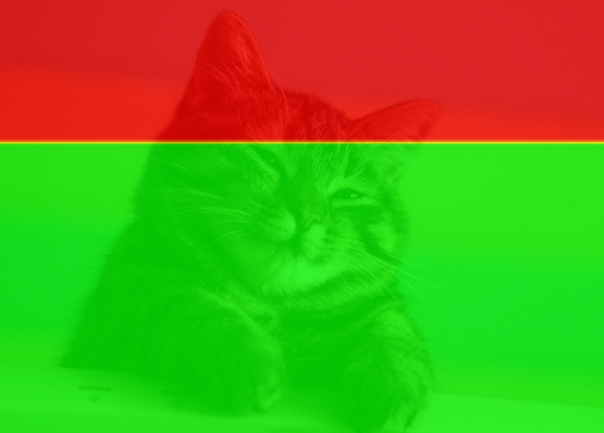
Exactly, isn't it?

Well, we got a mathematically justified attack, you can't fool math! Or…??

Shuffle dance

The idea is quite simple: write bits in order, and in random places. To do this, you need to take the PRNG, set it up to issue the same random flow with the same side (aka password). Without knowing the password, we will not be able to configure the PRNG and find the pixels in which the message is hidden. Test it on the cat.

Kitty (32% full):



His LSB:



The picture looks noisy, but not suspicious for an inexperienced analyst. What does Chi-square say?


It seems black hat won !? As if not so ...

Regularity-singularity

Another statistical method was Jessica Friedrich, Miroslav Golyan and Andreas Pfitstsman in 2001. It was named as the RS method. The original article can be found here.

The method contains several preparatory steps.

The image is divided into groups of n pixels. For example, 4 consecutive pixels in a row. As a rule, such groups contain adjacent pixels.
For our cat with sequential filling in the red channel, the first five groups will be:

• [78, 78, 79, 78]
  
• [78, 78, 78, 78]
  
• [78, 79, 78, 79]
  
• [79, 76, 79, 76]
  
• [76, 76, 76, 77]
  

(All measurements are in the classic RGB version)

Then we define the so-called discriminant function or smoothness function, which associates a true number to each group of pixels. The purpose of this function is to fix the smoothness or "regularity" of a group of pixels G. The noisier a group of pixels $$$G = (x_1, ..., x_n)$ the greater the discriminant function will be. The most common choice is the “variation” of a group of pixels or, more simply, the sum of the differences of neighboring pixels in a group. But also in it it is possible to consider statistical assumptions about the image.

$$

$$f (x_1, x_2, ..., x_n) = \ sum_ {i = 1} ^ {n-1} | x_ {i + 1} - x_i |$$

The smoothness function values ​​for a group of pixels from our example:

• f (78, 78, 79, 78) = 2
• f (78, 78, 78, 78) = 0
• f (78, 79, 78, 79) = 3
• f (79, 76, 79, 76) = 9
• f (76, 76, 76, 77) = 1

Next, the class of flipping functions from one pixel is determined.

They must have some properties.

$$

$$1. ~~~ \ forall x \ in P: ~ F (F (x)) = x, ~~ P = \ {0, ~ 255 \};$$

$$

$$2. ~~~ F_1: 0 \ leftrightarrow 1, ~ 2 \ leftrightarrow 3, ~ ..., 254 \ leftrightarrow 255;$$

$$

$$3. ~~~ \ forall x \ in P: ~ F _ {- 1} (x) = F_1 (x + 1) -1;$$

Where $$$F$ - any function from one class, $$$F_1$ - direct flipping function, and $$$F _ {- 1}$ - reverse. In addition, the identical flipping function is usually denoted. $$$F_0$ which does not change pixel.

The python flipping functions might look something like this:

 def flip(val): if val & 1: return val - 1 return val + 1 def invert_flip(val): if val & 1: return val + 1 return val - 1 def null_flip(val): return val 

For each group of pixels, we apply one of the flipping functions and, based on the value of the descriptive function before and after flipping, we determine the type of group of pixels: normal ( R egular), single / unusual ( S ingular), and useless unsuitable (unusable). Since the latter type is not used further, the method was named after the first letters of the key types. That's the whole secret of the name, singularity has nothing to do with it :)



We may want to apply different flipping to different pixels, for this we define a mask M with n values ​​of -1, 0 or 1.

$$

$$F_M (G) = (F_ {M (1)} (x_1), F_ {M (2)} (x_2), ..., F_ {M (n)} (x_n))$$

Let the mask for our example be classical - [1, 0, 0, 1]. It was experimentally found that symmetrical masks that do not contain $$$F _ {- 1}$ . Also, the successful variants will be: [0, 1, 0, 1], [0, 1, 1, 0], [1, 0, 1, 0]. Apply flipping for groups from the example, calculate the smoothness value and determine the type of the group of pixels:

• $$$F_M$ (78, 78, 79, 78) = [79, 78, 79, 79];
  f (79, 78, 79, 79) = 2 = 2 = f (78, 78, 79, 78)
  Unusable group
  
  
• $$$F_M$ (78, 78, 78, 78) = [79, 78, 78, 79];
  f (79, 78, 78, 79) = 2> 0 = f (78, 78, 78, 78)
  Regular group
  
  
• $$$F_M$ (78, 79, 78, 79) = [79, 79, 78, 78];
  f (79, 79, 78, 78) = 1 <3 = f (78, 79, 78, 79) Singular group
  
  
• $$$F_M$ (79, 76, 79, 76) = [78, 76, 79, 77];
  f (78, 76, 79, 77) = 7 <9 = f (79, 76, 79, 76) Singular group
  
  
• $$$F_M$ (76, 76, 76, 77) = [77, 76, 76, 76];
  f (77, 76, 76, 76) = 1 = 1 = f (76, 76, 76, 77)
  Unusable group
  
  

Denote the number of regular groups for the mask M as $$$R_m$ (in percentages of all groups), and $$$S_m$ for singular groups.

Then $$$R_M + S_M \ leq 1$ and $$$R _ {- M} + S _ {- M} \ leq 1$ , for a negative mask (all components of the mask are multiplied by -1), since $$$R_M + S_M + U_M = 1$ , wherein $$$U_m$ may be empty. Similarly for a negative mask.

The basic statistical hypothesis is that in a typical image the expected value $$$R_m$ equal to $$$R _ {- M}$ and the same is true for $$$S_m$ and $$$S _ {- M}$ . This is proved by experimental data and some dances with a tambourine around the last feature of the flipping function.

$$

$$R_M \ cong S_M ~~~~ R _ {- M} \ cong S _ {- M}$$

Check it out on our little example? Given the small sample size, we can not confirm this hypothesis. Let's see what happens with the inverted mask: [-1, 0, 0, -1].

• F_M (78, 78, 79, 78) = [77, 78, 79, 77];
  f (77, 78, 79, 77) = 4> 2 = f (77, 78, 79, 77)
  Regular group
  
  
• F_M (78, 78, 78, 78) = [77, 78, 78, 77];
  f (77, 78, 78, 77) = 2> 0 = f (78, 78, 78, 78)
  Regular group
  
  
• F_M (78, 79, 78, 79) = [77, 79, 78, 80];
  f (77, 79, 78, 80) = 5> 3 = f (78, 79, 78, 79)
  Regular group
  
  
• F_M (79, 76, 79, 76) = [80, 76, 79, 75];
  f (80, 76, 79, 75) = 11> 9 = f (79, 76, 79, 76)
  Regular group
  
  
• F_M (76, 76, 76, 77) = [75, 76, 76, 78];
  f (75, 76, 76, 78) = 3> 1 = f (76, 76, 76, 77)
  Regular group
  
  

Well, everything is obvious.

However, the difference between $$$R_m$ and $$$S_m$ tend to zero as the length m of the embedded message increases and we get that $$$R_M \ cong S_M$ .

It's funny that randomization of the LSB plane has the opposite effect on $$$R _ {- M}$ and $$$S _ {- M}$ . Their difference increases with the length m of the embedded message. An explanation of this phenomenon can be found in the original article.

Here is the schedule $$$R_m$ , $$$S_m$ , $$$R _ {- M}$ and $$$S _ {- M}$ Depending on the number of pixels with inverted LSB, it is called the RS-chart. The x-axis is the percentage of pixels with inverted LSBs, the y-axis is the relative number of regular and singular groups with the M and -M masks, $$$M = [0 ~ 1 ~ 1 ~ 0]$ .



The essence of the RS-steganalysis method is to evaluate the four curves of the RS diagram and calculate their intersection using extrapolation. Suppose we have a stegocontainer with a message of unknown length p (as a percentage of pixels) embedded in the lower bits of randomly selected pixels (that is, using RandomLSB). Our initial measurements of the number of groups R and S correspond to points $$$R_M (p / 2)$ , $$$S_M (p / 2)$ , $$$R _ {- M} (p / 2)$ and $$$S _ {- M} (p / 2)$ . We take the points exactly half the length of the message, since the message is a random bitstream and, on average, as mentioned earlier, only one half of the pixels will be changed by embedding the message.

If we invert the LSB of all pixels in the image and calculate the number of R and S groups, we get four points $$$R_M (1-p / 2)$ , $$$S_M (1-p / 2)$ , $$$R _ {- M} (1-p / 2)$ and $$$S _ {- M} (1-p / 2)$ . Since these two points depend on the specific randomization of LSB, we must repeat this process many times and evaluate $$$R_m (1/2)$ and $$$S_M (1/2)$ from statistical samples.

We can conditionally draw straight lines $$$R _ {- M} (p / 2)$ , $$$R _ {- M} (1-p / 2)$ and $$$S _ {- M} (p / 2)$ , $$$S _ {- M} (1-p / 2)$ .

Points $$$R_M (p / 2)$ , $$$R_m (1/2)$ , $$$R_M (1-p / 2)$ and $$$S_M (p / 2)$ , $$$S_m (1/2)$ , $$$S_M (1-p / 2)$ define two parabolas. Each parabola and the corresponding line intersect on the left. The arithmetic mean of the x-coordinates of both intersections makes it possible to estimate the unknown length of the message p.

To avoid a long statistical evaluation of the midpoints RM (1/2) and SM (1/2), you can take a couple more considerations:

1. Curve Intersection Point $$$R_m$ and $$$R _ {- M}$ has the same x coordinate as the intersection point for curves $$$S_m$ and $$$S _ {- M}$ . This is essentially a more stringent version of our statistical hypothesis. (see above)
2. The RM and SM curves intersect at m = 50%, or $$$R_M (1/2) = S_M (1/2)$ .

These two assumptions allow us to obtain a simple formula for the length of the secret message p. After scaling the x axis, so that p / 2 becomes 0, and 1 - p / 2 becomes equal to 1, the x-coordinate of the intersection point is the root of the following quadratic equation



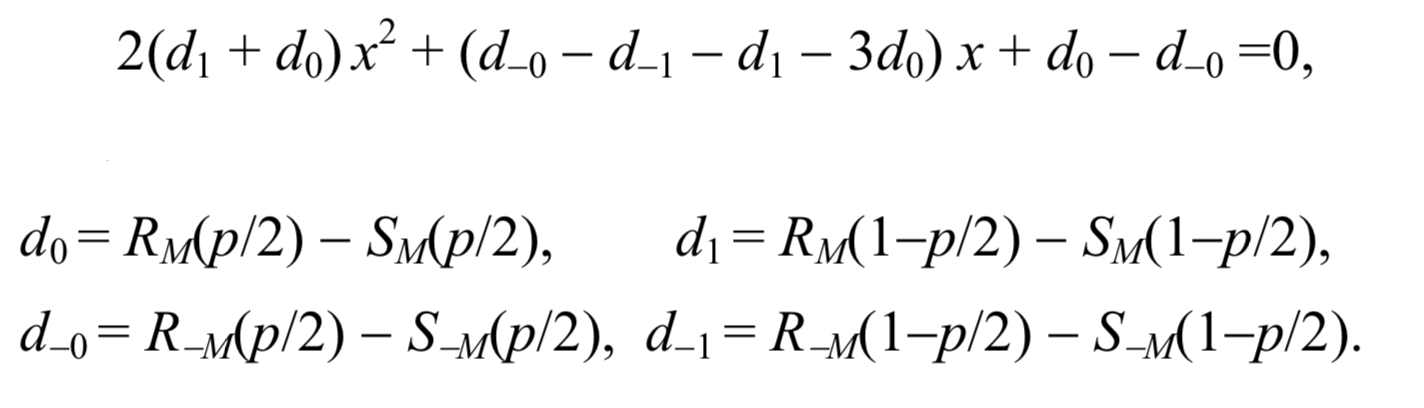
Then the message length can be calculated by the formula:

$$

$$p = \ frac {x} {x- \ frac {1} {2}}$$

Here our cat comes on the scene. (Is it time to give him a name?)

So, we have:

• Regular groups of RM (p / 2): 23121 pcs.
• Singular groups of SM (p / 2): 14,124 pcs.
• Regular groups with inverted RM mask (p / 2): 37191 pcs.
• Singular groups with inverted SM mask (p / 2): 8440 pcs.
• Regular groups with inverted LSB RM (1-p / 2): 20298 pcs.
• Singular groups with inverted LSB SM (1-p / 2): 16206 pcs.
• Regular groups with inverted LSB and inverted RM mask (1-p / 2): 40603 pcs.
• Singular groups with inverted LSB and inverted SM mask (1-p / 2): 6947 pcs.

(If you have a lot of free time, you can calculate them yourself, but for now I suggest you believe my calculations)

On the agenda we have one naked mathematics. Still remember how to solve quadratic equations?

$$

$$d_0 = $ 899$$

$$

$$d _ {- 0} = 28751$$

$$

$$d_1 = 4092$$

$$

$$d _ {- 1} = $ 3365$$

Substituting all d into the formula above, we obtain a quadratic equation, which we solve as taught in school.

$$

$$26178x ^ 2-35988x - 19754 = 0$$

$$

$$D = (-35988) ^ 2 - 426178 * (- 19754) = $ 336361699$$

$$

$$x_1 = 1.7951 ~~~~~~~~ x_2 = -0.4204$$

Take a smaller root, i.e. $$$x_2$ . Then the rough estimate for the message embedded in the cat will be:

$$

$$p = \ frac {-0.4204} {- 0.4204 - 0.5} = $ 0.456$$

Yes, this method has one big plus and one big minus. The advantage is that the method works with both conventional LSB-steganography and RandomLSB-steganography. Chi-square can not boast of such an opportunity. Our random kitten method recognized exactly and gave an estimate of the message length of 0.3256, which is very, very accurate.

The minus is in the large (very large) errors of this method, which grows along with the length of the message with sequential embedding . For example, for a cat with a fullness of 30%, my implementation of the method gives an approximate average estimate for three channels of 0.4633 or 46% of the total capacity, with a fullness of more than 95% - 0.8597. But for an empty cat already 0.0054. And this is a general trend, not dependent on implementation. The most accurate results with the usual LSB method gives a message with an embedded message length of 10% + - 5%.

Plus or minus

In order not to get caught, one must be unexpected and use ± 1 coding. Instead of changing the least significant bit in a byte of color, we will either increase the entire byte or decrease it by one. There are only two exceptions:

• we cannot reduce zero, therefore we will increase it,
  
• we also cannot increase 255, so we will always decrease this value.
  

For all other byte values, we completely randomly choose either a one or two increase. On top of this manipulation, the LSB will change as it did before. For greater reliability, it is better to take random bytes to write the message.

Here is our friend cat:



Externally, the implementation is imperceptible exactly for the same reason, why the differences between (0, 0, 0) and (1, 1, 1) were not visible.



The LSB slice remains just noisy due to writing to random places.



The chi-square is still blind, and the RS-method gives a rough estimate of 0.0036 .

To not very happy, read here this article.

The most attentive question may arise, how can we get a message if whole bytes change randomly, and we don’t have a password to insist the PRNG (it is better to use different aka generator state aka passwords to work with RandomLSB and ± 1 encoding). The answer is as simple as possible. We get the message in the same way as we did without ± 1 coding. We generally may not know about its use. I repeat, we use this trick only to bypass automatic detection tools . When inserting / retrieving a message, we work only with its LSB and nothing more. However, when detecting, we need to take into account the context of implementation, that is, all the bytes of the image in order to build statistical estimates. That’s what the whole ± 1 coding success is all about.

Instead of conclusion

Another very good attempt to use statistics against LSB-steganography was made in a method called Sample Pairs. You can find it here. His presence here would have made the article too academic, so I leave it to those interested in extracurricular reading. But anticipating questions from the audience, I will answer immediately: no, he does not catch ± 1 coding.

And of course machine learning. Modern ML-based methods give very good results. You can read about it here and here .

Based on this article, a small tool has been written (so far). It can generate data, perform a visual attack separately by channels, calculate the RS, SPA score and visualize the Chi-square results. And she is not going to stop there.

To summarize, I want to give a couple of tips:

• Embed the message in random bytes.
• Minimize the amount of information being introduced (remember Uncle Hamming).
• Use ± 1 coding.
• Choose pictures with noisy LSB.
• UPD from remzalp : Use nowhere not appear images.
• Be good!

I would be glad to see your suggestions, additions, corrections and other feedback!

PS I want to express special thanks to PavelMSTU for advice and motivational kicks.