How much data for learning model (not) similar to the test sample?
Consider one of the scenarios in which your machine learning model may be useless.
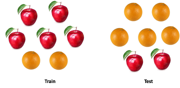
There is a saying: "Do not compare apples with oranges . " But what if you need to compare one set of apples with oranges with another, but the distribution of fruits in two sets is different? Can you work with the data? And how will you do it?
In real-life cases, this situation is ubiquitous. When developing machine learning models, we are faced with a situation where our model works well with the training sample, but the quality of the model drops sharply on test data.
')
And this is not about retraining. Suppose that we have built a model that gives an excellent result for cross-validation, but shows a poor result on the test. So in the test sample there is information that we do not take into account.
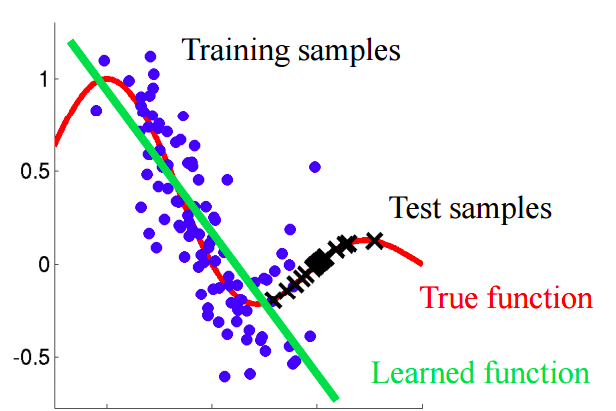
Imagine a situation in which we predict customer behavior in the store. If the training and test sample looks like the image below, this is a clear problem:

In this example, the model is trained on the data with the average value of the sign “customer age” lower than the average value of the same sign on the test. In the process of learning, the model has never “seen” the larger values of the sign “age”. If age is an important feature for a model, then one should not expect good results on the test sample.
In this text we will talk about "naive" approaches that allow to identify such phenomena and try to eliminate them.
We give a more accurate definition of this concept. Covariance refers to the values of features, and by covariant shift is meant the situation when the distributions of feature values in the training and test samples have different characteristics (parameters).
In real problems with a large number of variables, the covariant shift is difficult to detect. The article discusses the method of identifying and also taking into account the covariant shift in the data.
If there is a shift in the data, then when mixing two samples, we will be able to build a classifier that can determine whether an object belongs to a training or test sample.
Let's understand why this is so. Let us return to the example with customers, where age was a “shifted” sign of a training and test sample. If we take a classifier (for example, on the basis of a random forest) and try to divide the mixed sample into training and test, then age will be a very important feature for such a classification.

Let's try to apply the described idea to a real dataset. Use dataset from Kaggle competition.
First of all, let's perform a series of standard steps: clean, fill in the blanks, perform label encoding for categorical features. For the dataset in question, the step was not required, so let's skip its description.
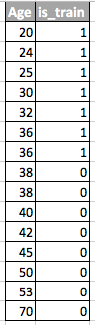
To both parts of the dataset - training and test - it is necessary to add a new indicator indicator. For the training sample with the value "1", for the test, respectively, "0".
Now it is necessary to combine two datasets. Because the training dataset contains a column of target values 'target', which is not in the test dataset, this column must be deleted.
For classification purposes, we will use the Random Forest Classifier, which we will configure to predict the labels of the data source in the combined dataset. You can use any other classifier.
We use a stratified randomized split into 4 folds. This way we will keep the ratio of the 'is_train' tags in each fold as in the original merged sample. For each splitting, we will train the classifier on most of the splitting and predict the class label for the smaller deferred part.
We calculate the value of the ROC AUC metric for our classifier. Based on this value, we conclude how well our classifier detects a covariant shift in the data.
If the classifier with well separates objects into training and test datasets, then the value of the ROC AUC metric should be significantly greater than 0.5, ideally close to 1. This picture indicates a strong covariant shift in the data.
Find the ROC AUC value:
The resulting value is close to 0.5. This means that our quality classifier is the same as the random predictor of tags. There is no evidence of a covariant shift in the data.
Since it’s taken from Kaggle, the result is pretty predictable. As in other machine learning competitions, the data are carefully checked to ensure that there are no shifts.
But such an approach can be applied in other data science problems to check for the presence of a covariant shift just before the start of the solution.
So, either we are seeing a covariant shift, or not. What to do to improve the quality of the model on the test?
Note: the method is applicable if there is a covariant shift in the data.

This algorithm will remove the signs from the red basket on the chart.
Note: the method is applicable regardless of whether there is a covariant shift in the data.
Let's look at the predictions we received in the previous section. For each object, the prediction contains the probability that this object belongs to the training set for our classifier.
For example, for the first object, our Random Forest Classifier considers that it belongs to the training set with a probability of 0.397. Let's call this value . Or you can say that the probability of belonging to the test data is 0.603. Similarly, let's call the probability .
Now a little trick: for each object of the training dataset, we calculate the coefficient .
Coefficient tells us how close the object from the training set is to the test data. Main thought:
We can use as weights in any of the models, in order to increase the weight of those observations that look similar to the test sample. Intuitively, this makes sense, since our model will be more data-oriented as in the test set.
These weights can be calculated using the code:
The resulting coefficients can be transferred to the model, for example, as follows:

A couple of words about the resulting histogram:
We hope that this post will help you in identifying the "covariant shift" in the data and in dealing with it.
[1] Shimodaira, H. (2000). The log-likelihood function. Journal of Statistical Planning and Inference, 90, 227–244.
[2] Bickel, S. et al. (2009). Discriminative Learning Under Covariate Shift. Journal of Machine Learning Research, 10, 2137–2155
[3] github.com/erlendd/covariate-shift-adaption
[4] Link to dataset used
PS Notebook with code from the article can be viewed here .
There is a saying: "Do not compare apples with oranges . " But what if you need to compare one set of apples with oranges with another, but the distribution of fruits in two sets is different? Can you work with the data? And how will you do it?
In real-life cases, this situation is ubiquitous. When developing machine learning models, we are faced with a situation where our model works well with the training sample, but the quality of the model drops sharply on test data.
')
And this is not about retraining. Suppose that we have built a model that gives an excellent result for cross-validation, but shows a poor result on the test. So in the test sample there is information that we do not take into account.
Imagine a situation in which we predict customer behavior in the store. If the training and test sample looks like the image below, this is a clear problem:
In this example, the model is trained on the data with the average value of the sign “customer age” lower than the average value of the same sign on the test. In the process of learning, the model has never “seen” the larger values of the sign “age”. If age is an important feature for a model, then one should not expect good results on the test sample.
In this text we will talk about "naive" approaches that allow to identify such phenomena and try to eliminate them.
Covariant shift
We give a more accurate definition of this concept. Covariance refers to the values of features, and by covariant shift is meant the situation when the distributions of feature values in the training and test samples have different characteristics (parameters).
In real problems with a large number of variables, the covariant shift is difficult to detect. The article discusses the method of identifying and also taking into account the covariant shift in the data.
main idea
If there is a shift in the data, then when mixing two samples, we will be able to build a classifier that can determine whether an object belongs to a training or test sample.
Let's understand why this is so. Let us return to the example with customers, where age was a “shifted” sign of a training and test sample. If we take a classifier (for example, on the basis of a random forest) and try to divide the mixed sample into training and test, then age will be a very important feature for such a classification.
Implementation
Let's try to apply the described idea to a real dataset. Use dataset from Kaggle competition.
Step 1: Data Preparation
First of all, let's perform a series of standard steps: clean, fill in the blanks, perform label encoding for categorical features. For the dataset in question, the step was not required, so let's skip its description.
import pandas as pd # train test train = pd.read_csv('train.csv',low_memory=True) test = pd.read_csv('test.csv',low_memory=True) Step 2: Add Data Source Indicator
To both parts of the dataset - training and test - it is necessary to add a new indicator indicator. For the training sample with the value "1", for the test, respectively, "0".
# , test, train test['is_train'] = 0 train['is_train'] = 1 Step 3: Combine Training and Test Samples
Now it is necessary to combine two datasets. Because the training dataset contains a column of target values 'target', which is not in the test dataset, this column must be deleted.
# train, test df_combine = pd.concat([train, test], axis=0, ignore_index=True) # target df_combine = df_combine.drop('target', axis =1) y = df_combine['is_train'].values # x = df_combine.drop('is_train', axis=1).values # tst, trn = test.values, train.values Step 4: building and testing the classifier
For classification purposes, we will use the Random Forest Classifier, which we will configure to predict the labels of the data source in the combined dataset. You can use any other classifier.
from sklearn.ensemble import RandomForestClassifier import numpy as np rfc = RandomForestClassifier(n_jobs=-1, max_depth=5, min_samples_leaf = 5) predictions = np.zeros(y.shape) # We use a stratified randomized split into 4 folds. This way we will keep the ratio of the 'is_train' tags in each fold as in the original merged sample. For each splitting, we will train the classifier on most of the splitting and predict the class label for the smaller deferred part.
from sklearn.model_selection import StratifiedKFold, cross_val_score skf = StratifiedKFold(n_splits=4, shuffle=True, random_state=100) for fold, (train_idx, test_idx) in enumerate(skf.split(x, y)): X_train, X_test = x[train_idx], x[test_idx] y_train, y_test = y[train_idx], y[test_idx] rfc.fit(X_train, y_train) probs = rfc.predict_proba(X_test)[:, 1] # predictions[test_idx] = probs Step 5: Interpret Results
We calculate the value of the ROC AUC metric for our classifier. Based on this value, we conclude how well our classifier detects a covariant shift in the data.
If the classifier with well separates objects into training and test datasets, then the value of the ROC AUC metric should be significantly greater than 0.5, ideally close to 1. This picture indicates a strong covariant shift in the data.
Find the ROC AUC value:
from sklearn.metrics import roc_auc_score print('ROC-AUC:', roc_auc_score(y_true=y, y_score=predictions)) # ROC-AUC: 0.49974692698385287 The resulting value is close to 0.5. This means that our quality classifier is the same as the random predictor of tags. There is no evidence of a covariant shift in the data.
Since it’s taken from Kaggle, the result is pretty predictable. As in other machine learning competitions, the data are carefully checked to ensure that there are no shifts.
But such an approach can be applied in other data science problems to check for the presence of a covariant shift just before the start of the solution.
Further steps
So, either we are seeing a covariant shift, or not. What to do to improve the quality of the model on the test?
- Remove offset features
- Use object importance weights based on density coefficient estimate
Removing displaced features:
Note: the method is applicable if there is a covariant shift in the data.
- Extract the importance of signs from the Random Forest Classifier classifier, which we have built and trained earlier.
- The most important features are those that are shifted and cause a shift in the data.
- Starting with the most important ones, delete by one feature, build the target model and look at its quality. Collect all signs for which the quality of the model is not reduced.
- Discard the collected signs from the data and build the final model.
This algorithm will remove the signs from the red basket on the chart.
Using object importance weights based on density coefficient estimation
Note: the method is applicable regardless of whether there is a covariant shift in the data.
Let's look at the predictions we received in the previous section. For each object, the prediction contains the probability that this object belongs to the training set for our classifier.
predictions[:10] #array([0.39743827 ... For example, for the first object, our Random Forest Classifier considers that it belongs to the training set with a probability of 0.397. Let's call this value . Or you can say that the probability of belonging to the test data is 0.603. Similarly, let's call the probability .
Now a little trick: for each object of the training dataset, we calculate the coefficient .
Coefficient tells us how close the object from the training set is to the test data. Main thought:
We can use as weights in any of the models, in order to increase the weight of those observations that look similar to the test sample. Intuitively, this makes sense, since our model will be more data-oriented as in the test set.
These weights can be calculated using the code:
import seaborn as sns import matplotlib.pyplot as plt plt.figure(figsize=(20,10)) predictions_train = predictions[len(tst):] weights = (1./predictions_train) - 1. weights /= np.mean(weights) # plt.xlabel(' w') plt.ylabel(' ') sns.distplot(weights, kde=False) The resulting coefficients can be transferred to the model, for example, as follows:
rfc = RandomForestClassifier(n_jobs=-1,max_depth=5) m.fit(X_train, y_train, sample_weight=weights) A couple of words about the resulting histogram:
- Larger weights correspond to observations more similar to the test sample.
- Almost 70% of the objects from the training sample have a weight close to 1, and, therefore, are in a subspace that is equally similar to the training and the test sample. This corresponds to the AUC value that we calculated earlier.
Conclusion
We hope that this post will help you in identifying the "covariant shift" in the data and in dealing with it.
Links
[1] Shimodaira, H. (2000). The log-likelihood function. Journal of Statistical Planning and Inference, 90, 227–244.
[2] Bickel, S. et al. (2009). Discriminative Learning Under Covariate Shift. Journal of Machine Learning Research, 10, 2137–2155
[3] github.com/erlendd/covariate-shift-adaption
[4] Link to dataset used
PS Notebook with code from the article can be viewed here .
Source: https://habr.com/ru/post/422185/
All Articles