AI, practical course. Configure the model and hyperparameters to recognize emotions in images

In previous articles of this training series, possible options for data preparation were described. Preprocessing and addition of data with images , also in these articles a Basic model of emotion recognition based on convolutional neural network images was built.
In this article, we will build an improved convolutional neural network model for recognizing emotions in images using a technique called inductive learning .

First you need to read the article on the Basic Model of Emotion Recognition on Images , you can also refer to it during the reading, since some sections, including the study of source data and the description of network indicators, will not be given here in detail.

Data

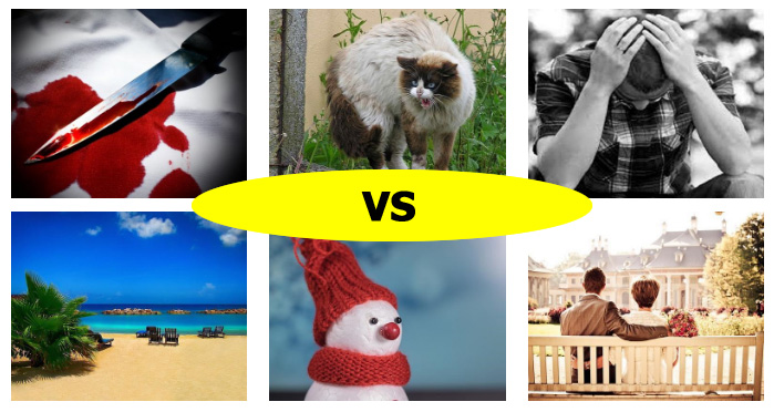
The data set contains 1630 images with emotions of two classes: Negative (class 0) and Positive (class 1). A few examples of such images are shown below.
')
Negative






Positive






Some of the examples contain an obvious positive or negative emotion, while others may not be classified - even with human participation. Based on a visual check of such cases, we estimate that the maximum possible accuracy should be about 80 percent. Note that the random classifier provides approximately 53 percent accuracy due to a small imbalance of classes.

To train the model, we use the technique of holding part of the samples and divide the initial data set into two parts, one of which (20 percent of the initial set) will be used by us for testing. Partitioning is performed using stratification : this means that the balance between classes is maintained in the training and test sets.

Solving the problem of insufficient data

The base model demonstrated results, only slightly better random class prediction of images. There may be many possible reasons for this behavior. We believe that the main reason is that the available amount of data is decidedly insufficient for such training of the convolutional part of the network, which would allow to obtain the characteristics based on the input image.
There are many different ways to solve the problem of data failure. Here are a few of them:

• Re-sample The idea of ​​the method is to evaluate the distribution of data and select new examples from this distribution.
• Teaching without a teacher . Everyone can find large amounts of data of the same nature as the labeled examples in a given data set. For example, it can be movies for video recognition or audio books for speech recognition. The next step on this path is to use this data for preliminary training of the model (for example, with the help of autocoders).
• Data augmentation . During this process, the sample data is modified randomly using a given set of transforms.
• Inductive learning . This topic is of great interest to us, so let's take a look at it in more detail.

Inductive learning

The term inductive learning refers to a set of techniques that use models (often very large) that are trained on different data sets of approximately the same nature.





Comparison of traditional machine learning and inductive learning methods. The image is taken from S. Ruder 's blog post “What is inductive learning?” .
There are three main scenarios for the use of inductive learning:

• Pre-trained models . Any user can simply take a model trained by someone else and use it for their tasks. Such a scenario is possible if the tasks are very similar.
• The block selection features . At this point, we know that the architecture of the model can be divided into two main parts: The feature extraction unit , which is responsible for selecting features from the input data, and the classification module , which classifies examples based on the features obtained. Usually, the feature extraction unit is the main part of the model. The idea of ​​the method is to take a block of feature extraction from a model trained in another task, fix its weights (make them obsolete), and then build on its basis new classification modules for the problem in question. The classification module is usually not very deep and consists of several fully connected layers, so this model is much easier to train.
• Accurate and deep tuning . This method is like a script using the feature selection block. The same actions are performed with the exception of “freezing” the feature extraction unit. For example, you can take the VGG network as a feature selection block and freeze only the first three (out of four) convolutional blocks in it. In this case, the feature extraction unit can better adapt to the current task. For more information, see F. Chollet's blog entry. Building powerful image classification models using a very small amount of data .

A detailed description of the scenarios for the use of inductive learning can be found in the Stanford University course Convolutional neural networks CS231n for visual recognition by Fei-Fei Li and S. Ruder's blog entry (S. Ruder) Inductive learning is the next milestone in development machine learning (the subject is considered more comprehensively).

You may have questions: why are all these methods needed and why can they work? We will try to answer them.

• The benefits of using large data sets. For example, we can take a feature extraction block from a model trained on 14 million images contained in the ImageNet contest dataset. These models are complex enough to ensure the selection of very high-quality features from the input data.
• Considerations related to time. Training large models can take weeks or even months. In this case, everyone can save a huge amount of time and computing resources .
• The weighty assumption underlying why all this can work is as follows: Signs obtained as a result of training in one task may be useful and suitable for another task. In other words, signs have the property of invariance with respect to a problem. Please note that the domain of the new task should be similar to the domain of the original task. Otherwise, the feature extraction unit may even worsen the results obtained.

Advanced Model Architecture

Now we are familiar with the concept of inductive learning. We also know that ImageNet is a major event, in which almost all modern advanced architecture of convolutional neural networks were tested. Let's try to take a feature extraction block from one of these networks.

Fortunately, the Keras library provides us with several pre-trained (within ImageNet) models that were created within this platform. We import and use one of these models.



In this case, we will use a network with a VGG architecture. To select only the feature selection block, remove the classification module (three upper fully connected layers) of the network by setting the include_top parameter to False . We also want to initialize our network with the weights of the network trained within ImageNet. The last parameter is the size of the input data.

Please note that the size of the original images in the ImageNet competition is (224, 224, 3), while our images are sized (400, 500, 3). However, we use convolutional layers — this means that the weights of the network are the weights of the sliding cores in the convolution operation. Coupled with the parameter sharing property (a discussion of this is found in our theoretical article Overview of convolutional neural networks for image classification ) - this leads to the fact that the size of the input data can be almost arbitrary, since the convolution is performed by means of a sliding window, and this window can slide image of arbitrary size. The only limitation is that the size of the input data must be large enough so that it does not collapse into one point (spatial dimensions) in any intermediate layer, since otherwise it will be impossible to perform further calculations.

Another trick we use is caching . VGG is a very large network. One straight pass for all images (1630 examples) through the feature extraction block takes approximately 50 seconds. However, it should be remembered that the weights of the feature extraction block are fixed, and a straight pass always gives the same result for the same image. We can use this fact to perform a direct pass through the feature extraction block only once and then cache the results in the intermediate array. To implement this scenario, we first create an instance of the ImageDataGenerator class to load files from the hard disk directly (for more information, see the basic article Basic Model of Emotion Recognition in Images ).



In the next step, in the prediction mode, we use the previously created feature extraction block in the model to obtain the image features.



It takes about 50 seconds. Now we can use the results for a very fast learning of the upper classification part of the model - one epoch lasts about 1 second. Imagine now that each epoch lasts 50 seconds longer. Thus, this simple caching method allowed us to speed up the process of network training by 50 times! In this scenario, we save all the signs for all the examples in the RAM, since its volume is enough for this. When using a larger data set, you can calculate the properties, write them to the hard disk, and then read them using the same approach associated with the generator class.

Finally, consider the architecture of the classification part of the model:





Recall that a four-dimensional tensor (examples, height, width, and channels) is output at the output of a feature extraction block of a convolutional neural network, and a two-dimensional tensor (examples, features) is taken for classification. One of the ways to transform a four-dimensional tensor with attributes is simply its alignment around the last three axes (we used a similar technique in the basic model). In this scenario, we use a different approach, called global average - based subsampling (GAP). Instead of aligning four-dimensional vectors, we will take an average based on two spatial dimensions. In fact, we take a feature map and just average all the values ​​in it. The GAP method was first introduced in the excellent work of Min Lin (Min Lin) Network in a network (this book is really worth exploring it, because it covers some important concepts - for example, convolutions of 1 × 1 size). One of the obvious advantages of the GAP approach is a significant reduction in the number of parameters. When using GAP, we get only 512 signs for each example, while aligning the raw data, the number of signs will be 15 × 12 × 512 = 92 160. This can lead to serious overhead, since in this case the classification part of the model will have about 50 millions of options! Other elements of the classification part of the model, such as fully connected layers and layers that implement the exclusion method, are discussed in detail in the article Basic Model of Emotion Recognition in Images .

Settings and learning options

After we have prepared the architecture of our model with the help of Keras, it is necessary to configure the entire model for training using the compilation method.



In this case, we use settings that are almost the same as those of the base model, with the exception of the choice of optimizer. To optimize learning, binary cross entropy will be used as a loss function, and an accuracy metric will additionally be tracked. We use the Adam method as an optimizer. Adam is a type of stochastic gradient descent algorithm with momentum and adaptive learning rate (for more information, see the blog post by S. Ruder Review of gradient descent optimization algorithms ).

The learning rate is an optimizer hyperparameter that must be configured to ensure that the model works. Recall what the formula for “vanilla” gradient descent looks like, which does not contain additional functionality:



Θ is the vector of model parameters (in our case, weights of the neural network), £ is the objective function, ∇ is the gradient operator (calculated using the error back-propagation algorithm), α is the learning rate. Thus, the gradient of the objective function is the direction of the optimization step in the parameter space, and the learning rate is its size. When using an unreasonably high learning rate, there is a chance that the optimal point will constantly slip over due to an excessively large step size. On the other hand, if the learning rate is too low, then the optimization will take too much time and can provide convergence only in low-quality local minima instead of global extremum. Therefore, in each specific situation it is necessary to seek an appropriate compromise. Using the default settings for the Adam algorithm is a good starting point to get started.

However, in this task, the default Adam settings show poor results. We need to reduce the initial learning rate to a value of 0.0001. Otherwise, the training will not be able to provide convergence.

Ultimately, we can start learning for 100 epochs and then save the model and the history of learning. The % time command is an Ipython * magic command that allows you to measure code execution time.

Evaluation

Let's evaluate the effectiveness of the model during training. In our case, the verification accuracy is 73 percent (compared to 55 percent when using the base model). This result is much better than the base model.

Let's also look at the distribution of errors using a matrix of inaccuracies. Errors are distributed almost evenly between the classes with a slight shift toward incorrectly classified negative examples (upper left cell of the inaccuracy matrix). This can be explained by a small imbalance in the data set towards a positive class.

Another metric we track is the receiver performance curve (ROC curve) and the area under this curve (AUC). For a detailed description of these metrics, see the article Basic Model of Emotion Recognition in Images .



The closer the ROC curve is to the upper left of the graph and the larger the area under it (AUC metric), the better the classifier works. This figure clearly shows that the improved and pre-trained model demonstrates better results than the basic model created from scratch. The AUC value for a pre-trained model is 0.82, which is a good result.

Conclusion

In this article, we met with a powerful technique - inductive learning. We also built a convolutional neural network classifier using a pre-trained feature extraction block based on the VGG architecture. This classifier has surpassed the basic convolutional model trained from scratch in terms of its performance. The gain was exactly 18 percent, and the gain in the AUC metric was 0.25, which demonstrates a very significant improvement in the quality of the system.