How we reduced the time to develop scoring models five times by switching to Python

Now everyone is talking a lot about artificial intelligence and its application in all areas of the company. However, there are some areas where one type of model has dominated since ancient times, the so-called “white box” - logistic regression. One such area is bank credit scoring.
There are several reasons for this:
- Regression coefficients can be easily explained in contrast to “black boxes” like boosting, which can include more than 500 variables.
- Machine learning is still not credible to management because of the difficulty in interpreting models.
- There are unwritten requirements of the regulator for the interpretability of models: at any time, for example, the Central Bank may ask for an explanation - why the loan was denied to the borrower
- Companies use external data mining programs (for example, rapid miner, SAS Enterprise Miner, STATISTICA or any other package), which allow you to quickly learn how to build models, even without programming skills
These reasons make it almost impossible to use complex machine learning models in some areas, so it is important to be able to “squeeze the most” out of a simple logistic regression that is easy to explain and interpret.
')
In this post, we will describe how, when building scoring, we abandoned external data mining packages in favor of an open source solution in the form of Python, increased development speed several times, and also improved the quality of all models.
Scoring process
The classic process of building scoring models on a regression is as follows:
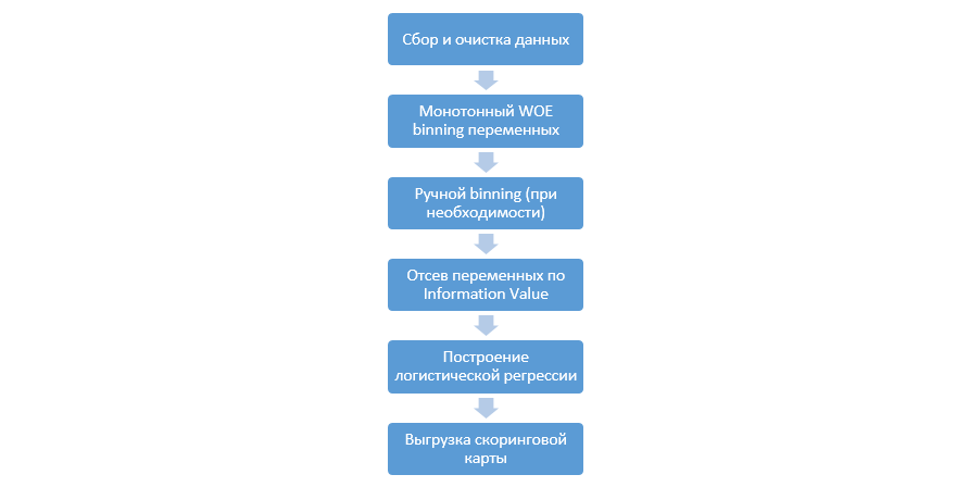
It may vary from company to company, but the main stages remain constant. We always need to produce binning variables (as opposed to the machine learning paradigm, where in most cases only categorical coding is needed), eliminating them by the Information Value (IV), and manually unloading all coefficients and bins for DSL integration.
This approach to building scoring cards worked fine in the 90s, but the technology of classical data mining packages is very outdated and does not allow the use of new techniques, such as, for example, L2 regularization in regression, which can significantly improve the quality of models.
At one point, as a study, we decided to reproduce all the steps that analysts do in building scoring, supplement them with knowledge of Data Scientists, and also automate the entire process as much as possible.
Python Upgrade
As a development tool, we chose Python for its simplicity and good libraries, and began to reproduce all the steps in order.
The first step is to collect data and generate variables - this stage is a significant part of the work of analysts.
In Python, you can load the collected data from the database using pymysql.
Code to download from the database
def con(): conn = pymysql.connect( host='10.100.10.100', port=3306, user='******* ', password='*****', db='mysql') return conn; df = pd.read_sql(''' SELECT * FROM idf_ru.data_for_scoring ''', con=con()) Next, we replace the rare and missing values with a separate category to prevent ovefitting, select the target, delete the extra columns, and also divide by the train and test.
Data preparation
def filling(df): cat_vars = df.select_dtypes(include=[object]).columns num_vars = df.select_dtypes(include=[np.number]).columns df[cat_vars] = df[cat_vars].fillna('_MISSING_') df[num_vars] = df[num_vars].fillna(np.nan) return df def replace_not_frequent(df, cols, perc_min=5, value_to_replace = "_ELSE_"): else_df = pd.DataFrame(columns=['var', 'list']) for i in cols: if i != 'date_requested' and i != 'credit_id': t = df[i].value_counts(normalize=True) q = list(t[t.values < perc_min/100].index) if q: else_df = else_df.append(pd.DataFrame([[i, q]], columns=['var', 'list'])) df.loc[df[i].value_counts(normalize=True)[df[i]].values < perc_min/100, i] =value_to_replace else_df = else_df.set_index('var') return df, else_df cat_vars = df.select_dtypes(include=[object]).columns df = filling(df) df, else_df = replace_not_frequent_2(df, cat_vars) df.drop(['credit_id', 'target_value', 'bor_credit_id', 'bchg_credit_id', 'last_credit_id', 'bcacr_credit_id', 'bor_bonuses_got' ], axis=1, inplace=True) df_train, df_test, y_train, y_test = train_test_split(df, y, test_size=0.33, stratify=df.y, random_state=42) Now begins the most important stage in scoring for regression - you need to write WOE-binning for numeric and categorical variables. In the public domain, we did not find good and suitable options for us and decided to write it ourselves. They took this article of 2017 as the basis for numerical binning, as well as this , categorical, they wrote from scratch themselves. The results were impressive (Gini rose by 3–5 on the test compared with the binning algorithms of external data mining programs).
After that, you can look at the graphs or tables (which we later write to excel), how the variables were broken into groups and check the monotony:
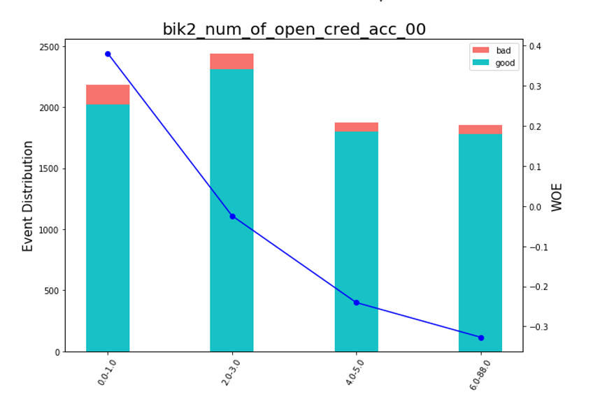
Drawing Bean Charts
def plot_bin(ev, for_excel=False): ind = np.arange(len(ev.index)) width = 0.35 fig, ax1 = plt.subplots(figsize=(10, 7)) ax2 = ax1.twinx() p1 = ax1.bar(ind, ev['NONEVENT'], width, color=(24/254, 192/254, 196/254)) p2 = ax1.bar(ind, ev['EVENT'], width, bottom=ev['NONEVENT'], color=(246/254, 115/254, 109/254)) ax1.set_ylabel('Event Distribution', fontsize=15) ax2.set_ylabel('WOE', fontsize=15) plt.title(list(ev.VAR_NAME)[0], fontsize=20) ax2.plot(ind, ev['WOE'], marker='o', color='blue') # Legend plt.legend((p2[0], p1[0]), ('bad', 'good'), loc='best', fontsize=10) #Set xticklabels q = list() for i in range(len(ev)): try: mn = str(round(ev.MIN_VALUE[i], 2)) mx = str(round(ev.MAX_VALUE[i], 2)) except: mn = str((ev.MIN_VALUE[i])) mx = str((ev.MAX_VALUE[i])) q.append(mn + '-' + mx) plt.xticks(ind, q, rotation='vertical') for tick in ax1.get_xticklabels(): tick.set_rotation(60) plt.savefig('{}.png'.format(ev.VAR_NAME[0]), dpi=500, bbox_inches = 'tight') plt.show() def plot_all_bins(iv_df): for i in [x.replace('WOE_','') for x in X_train.columns]: ev = iv_df[iv_df.VAR_NAME==i] ev.reset_index(inplace=True) plot_bin(ev) A separate function was written for manual binning, which is useful, for example, in the case of the variable "OS version", where all phones on Android and iOS were grouped manually.
Manual binning function
def adjust_binning(df, bins_dict): for i in range(len(bins_dict)): key = list(bins_dict.keys())[i] if type(list(bins_dict.values())[i])==dict: df[key] = df[key].map(list(bins_dict.values())[i]) else: #Categories labels categories = list() for j in range(len(list(bins_dict.values())[i])): if j == 0: categories.append('<'+ str(list(bins_dict.values())[i][j])) try: categories.append('(' + str(list(bins_dict.values())[i][j]) +'; '+ str(list(bins_dict.values())[i][j+1]) + ']') except: categories.append('(' + str(list(bins_dict.values())[i][j])) elif j==len(list(bins_dict.values())[i])-1: categories.append(str(list(bins_dict.values())[i][j]) +'>') else: categories.append('(' + str(list(bins_dict.values())[i][j]) +'; '+ str(list(bins_dict.values())[i][j+1]) + ']') values = [df[key].min()] + list(bins_dict.values())[i] + [df[key].max()] df[key + '_bins'] = pd.cut(df[key], values, include_lowest=True, labels=categories).astype(object).fillna('_MISSING_').astype(str) df[key] = df[key + '_bins']#.map(df.groupby(key + '_bins')[key].agg('median')) df.drop([key + '_bins'], axis=1, inplace=True) return df bins_dict = { 'equi_delinquencyDays': [ 200,400,600] 'loan_purpose': {'medicine':'1_group', 'repair':'1_group', 'helpFriend':'2_group'} } df = adjust_binning(df, bins_dict) The next step is the selection of variables on the Information Value. The standard value is a cut-off of 0.1 (all variables below do not have good predictive power).
After that a correlation check was performed. Of the two correlating variables, you need to remove the one that has IV less. Cut-off removal was taken 0.75.
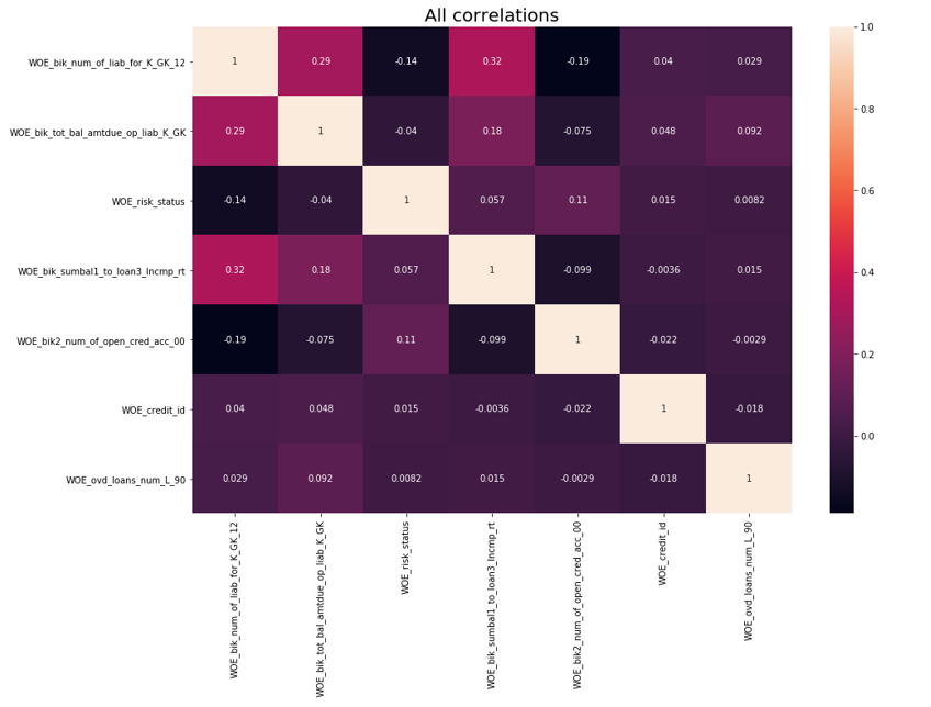
Removing correlations
def delete_correlated_features(df, cut_off=0.75, exclude = []): # Create correlation matrix corr_matrix = df.corr().abs() # Select upper triangle of correlation matrix upper = corr_matrix.where(np.triu(np.ones(corr_matrix.shape), k=1).astype(np.bool)) # Plotting All correlations f, ax = plt.subplots(figsize=(15, 10)) plt.title('All correlations', fontsize=20) sns.heatmap(X_train.corr(), annot=True) # Plotting highly correlated try: f, ax = plt.subplots(figsize=(15, 10)) plt.title('High correlated', fontsize=20) sns.heatmap(corr_matrix[(corr_matrix>cut_off) & (corr_matrix!=1)].dropna(axis=0, how='all').dropna(axis=1, how='all'), annot=True, linewidths=.5) except: print ('No highly correlated features found') # Find index of feature columns with correlation greater than cut_off to_drop = [column for column in upper.columns if any(upper[column] > cut_off)] to_drop = [column for column in to_drop if column not in exclude] print ('Dropped columns:', to_drop, '\n') df2 = df.drop(to_drop, axis=1) print ('Features left after correlation check: {}'.format(len(df.columns)-len(to_drop)), '\n') print ('Not dropped columns:', list(df2.columns), '\n') # Plotting final correlations f, ax = plt.subplots(figsize=(15, 10)) plt.title('Final correlations', fontsize=20) sns.heatmap(df2.corr(), annot=True) plt.show() return df2 In addition to the IV selection, we added a recursive search for the optimal number of variables using the RFE method from sklearn.
As we see in the graph, after 13 variables, the quality does not change, which means that the extra ones can be removed. For regression, more than 15 variables in scoring are considered bad tone, which in most cases is corrected using RFE.
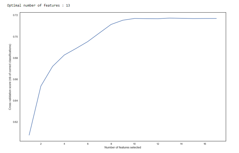
RFE
def RFE_feature_selection(clf_lr, X, y): rfecv = RFECV(estimator=clf_lr, step=1, cv=StratifiedKFold(5), verbose=0, scoring='roc_auc') rfecv.fit(X, y) print("Optimal number of features : %d" % rfecv.n_features_) # Plot number of features VS. cross-validation scores f, ax = plt.subplots(figsize=(14, 9)) plt.xlabel("Number of features selected") plt.ylabel("Cross validation score (nb of correct classifications)") plt.plot(range(1, len(rfecv.grid_scores_) + 1), rfecv.grid_scores_) plt.show() mask = rfecv.get_support() X = X.ix[:, mask] return X Next, a regression was constructed and its metrics were evaluated for cross-validation and test sampling. Usually everyone looks at the Gini coefficient (a good article about him is here ).
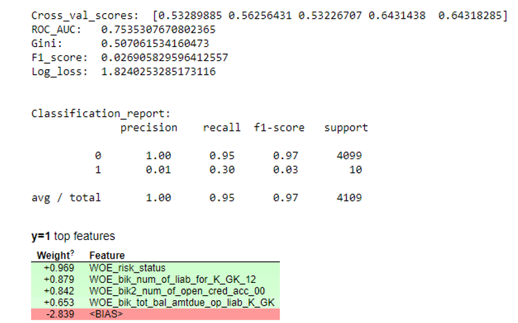
Simulation results
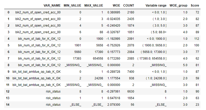
def plot_score(clf, X_test, y_test, feat_to_show=30, is_normalize=False, cut_off=0.5): #cm = confusion_matrix(pd.Series(clf.predict_proba(X_test)[:,1]).apply(lambda x: 1 if x>cut_off else 0), y_test) print ('ROC_AUC: ', round(roc_auc_score(y_test, clf.predict_proba(X_test)[:,1]), 3)) print ('Gini: ', round(2*roc_auc_score(y_test, clf.predict_proba(X_test)[:,1]) - 1, 3)) print ('F1_score: ', round(f1_score(y_test, clf.predict(X_test)), 3)) print ('Log_loss: ', round(log_loss(y_test, clf.predict(X_test)), 3)) print ('\n') print ('Classification_report: \n', classification_report(pd.Series(clf.predict_proba(X_test)[:,1]).apply(lambda x: 1 if x>cut_off else 0), y_test)) skplt.metrics.plot_confusion_matrix(y_test, pd.Series(clf.predict_proba(X_test)[:,1]).apply(lambda x: 1 if x>cut_off else 0), title="Confusion Matrix", normalize=is_normalize,figsize=(8,8),text_fontsize='large') display(eli5.show_weights(clf, top=20, feature_names = list(X_test.columns))) clf_lr = LogisticRegressionCV(random_state=1, cv=7) clf_lr.fit(X_train, y_train) plot_score(clf_lr, X_test, y_test, cut_off=0.5) When we are satisfied that the quality of the model suits us, we need to record all the results (regression coefficients, groups of beans, Gini stability graphs and variables, etc.) in excel. For this, it is convenient to use xlsxwriter, which can work with both data and pictures.
Exel sheet examples:
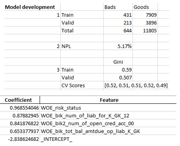
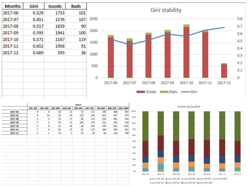
Write to excel
#WRITING writer = pd.ExcelWriter('PDL_Score_20180815-3.xlsx', engine='xlsxwriter') workbook = writer.book worksheet = workbook.add_worksheet('Sample information') bold = workbook.add_format({'bold': True}) percent_fmt = workbook.add_format({'num_format': '0.00%'}) worksheet.set_column('A:A', 20) worksheet.set_column('B:B', 15) worksheet.set_column('C:C', 10) # Sample worksheet.write('A2', 'Sample conditions', bold) worksheet.write('A3', 1) worksheet.write('A4', 2) worksheet.write('A5', 3) worksheet.write('A6', 4) # Model worksheet.write('A8', 'Model development', bold) worksheet.write('A9', 1) #labels worksheet.write('C8', 'Bads') worksheet.write('D8', 'Goods') worksheet.write('B9', 'Train') worksheet.write('B10', 'Valid') worksheet.write('B11', 'Total') # goods and bads worksheet.write('C9', y_train.value_counts()[1]) worksheet.write('C10', y_test.value_counts()[1]) worksheet.write('D9', y_train.value_counts()[0]) worksheet.write('D10', y_test.value_counts()[0]) worksheet.write('C11', y.value_counts()[1]) worksheet.write('D11', y.value_counts()[0]) # NPL worksheet.write('A13', 2) worksheet.write('B13', 'NPL') worksheet.write('C13', (y.value_counts()[1]/(y.value_counts()[1]+y.value_counts()[0])), percent_fmt) worksheet.write('A16', 3) worksheet.write('C15', 'Gini') worksheet.write('B16', 'Train') worksheet.write('B17', 'Valid') worksheet.write('B18', 'CV Scores') worksheet.write('C18', str([round(sc, 2) for sc in scores])) worksheet.write('C16', round(2*roc_auc_score(y_train, clf_lr.predict_proba(X_train)[:,1]) - 1, 3)) worksheet.write('C17', round(2*roc_auc_score(y_test, clf_lr.predict_proba(X_test)[:,1]) - 1, 3)) # Regreesion coefs feat.to_excel(writer, sheet_name='Regression coefficients', index=False) worksheet2 = writer.sheets['Regression coefficients'] worksheet2.set_column('A:A', 15) worksheet2.set_column('B:B', 50) #WOE ivs[['VAR_NAME', 'Variable range', 'WOE', 'COUNT', 'WOE_group']].to_excel(writer, sheet_name='WOE', index=False) worksheet3 = writer.sheets['WOE'] worksheet3.set_column('A:A', 50) worksheet3.set_column('B:B', 60) worksheet3.set_column('C:C', 30) worksheet3.set_column('D:D', 20) worksheet3.set_column('E:E', 12) for num, i in enumerate([x.replace('WOE_','') for x in X_train.columns]): ev = iv_df[iv_df.VAR_NAME==i] ev.reset_index(inplace=True) worksheet3.insert_image('G{}'.format(num*34+1), '{}.png'.format(i)) df3.to_excel(writer, sheet_name='Data', index=False) table.to_excel(writer, sheet_name='Scores by buckets', header = True, index = True) worksheet4 = writer.sheets['Scores by buckets'] worksheet4.set_column('A:A', 20) worksheet4.insert_image('J1', 'score_distribution.png') Ginis.to_excel(writer, sheet_name='Gini distribution', header = True, index = True) worksheet5 = writer.sheets['Gini distribution'] worksheet5.insert_image('E1', 'gini_stability.png') writer.save() The final excel at the end once again looks like management, and then given to IT to embed the model in production.
Total
As we have seen, almost all stages of scoring can be automated so that analysts do not need programming skills to build models. In our case, after creating this framework, the analyst is only required to collect data and specify several parameters (specify the target variable, which columns to delete, the minimum number of bins, the cut-off coefficient for correlation of variables, etc.), after which you can run the python script, who builds a model and gives excel with the desired results.
Of course, sometimes you have to correct the code for the needs of a specific project, and you will not manage to run a single script button while modeling, but even now we see the quality better than the packages used on data mining market thanks to such techniques as optimal and monotonous binning, correlation testing , RFE, regularized version of regression, etc.
Thus, thanks to the use of Python, we have significantly reduced the development time for scoring cards, as well as reduced labor costs for analysts.
Source: https://habr.com/ru/post/421091/
All Articles