Reinforcement training in PyBullet

Many who study machine learning are familiar with the OpenAI project, of which Ilon Mask is one of the founders, and use the OpenAI Gym platform as a medium to train their neural network models.

Gym contains a huge set of environments, some of them - various kinds of physical simulations: the movement of animals, humans, robots . These simulations are based on the MuJoCo physics engine, which is free for educational and scientific purposes.
')
In this article, we will create an extremely simple physical simulation similar to the OpenAI Gym environment, but based on the Bullet ( PyBullet ) free physics engine. And also create an agent to work with this environment.

PyBullet is a python module for creating a physical simulation environment based on the Bullet Physics engine. He, like MuJoCo, is quite often used as stimulation of various robots, who are interested in habr there is an article with real examples.

For PyBullet there is a pretty good QuickStartGuide , which contains links to examples on the page with the source code on GitHub .

PyBullet allows you to upload already created models in URDF, SDF or MJCF format. The source has a library of models in these formats, as well as fully prepared environments of simulators of real robots.

In our case, we ourselves will create an environment using PyBullet tools. The environment interface will be similar to the OpenAI Gym interface. In this way, we will be able to train our agents both in our environment and in the Gym environment.

All code (iPython), as well as the work of the program can be seen in the Google Laboratory .

Environment

Our environment will consist of a ball that can move along a vertical axis within a certain range of heights. The ball has a mass, and it is acted upon by gravity, and the agent must, by controlling the vertical force applied to the ball, bring it to the goal. Target height changes with every experience restart.



The simulation is very simple, and in fact can be considered as a simulation of some elementary propulsion.

Three methods are used to work with the environment: reset (restarting the experience and creating all the objects of the environment), step (applying the selected action and obtaining the resulting state of the environment), render (visual display of the environment).

When you initialize the environment, you need to connect our object to the physical simulation. Two connection options are possible: with a graphical interface (GUI) and without (DIRECT). In our case, this is DIRECT.

pb.connect(pb.DIRECT) 

reset

With each new experience, we reset the pb.resetSimulation () simulation and create all the environment objects again.

In PyBullet, objects have 2 forms: a collision shape ( Collision Shape ), and a visual shape ( Visual Shape ). The first is used by the physics engine to calculate collisions of objects and, to speed up the calculation of physics, usually has a simpler form than a real object. The second is optional, and is used only when forming an image of an object.

Forms are collected in a single object (body) - MultiBody . The body can be composed of one form (a pair of CollisionShape / Visual Shape ), as in our case, or several.

In addition to the forms that make up the body, it is necessary to determine its mass, position and orientation in space.


We will create 3 bodies: Ball, Plane (earth) and Pointer to the target. The last object will have only the form of visualization and zero mass, so it will not participate in the physical interaction between the bodies:

 #  floorColShape = pb.createCollisionShape(pb.GEOM_PLANE) #   (GEOM_PLANE), visualShape -    ,   GEOM_BOX floorVisualShapeId = pb.createVisualShape(pb.GEOM_BOX,halfExtents=[100,100,0.0001], rgbaColor=[1,1,.98,1]) pb_floorId = pb.createMultiBody(0,floorColShape,floorVisualShapeId, [0,0,0], [0,0,0,1]) #  PB_BallRadius = 0.2 PB_BallMass = 1 ballPosition = [0,0,5] ballOrientation=[0,0,0,1] ballColShape = pb.createCollisionShape(pb.GEOM_SPHERE,radius=PB_BallRadius) ballVisualShapeId = pb.createVisualShape(pb.GEOM_SPHERE,radius=PB_BallRadius, rgbaColor=[1,0.27,0,1]) pb_ballId = pb.createMultiBody(PB_BallMass, ballColShape, ballVisualShapeId, ballPosition, ballOrientation) #   TARGET_Z = 8 targetPosition = [0,0,TARGET_Z] targetOrientation=[0,0,0,1] targetVisualShapeId = pb.createVisualShape(pb.GEOM_BOX,halfExtents=[1,0.025,0.025], rgbaColor=[0,0,0,1]) pb_targetId = pb.createMultiBody(0,-1, targetVisualShapeId, targetPosition, targetOrientation) 

Determine the gravity and time step of the simulation.

 pb.setGravity(0,0,-10) pb.setTimeStep(1./60) 

In order for the ball not to fall immediately after running the simulation, we balance gravity.

 pb_force = 10 * PB_BallMass pb.applyExternalForce(pb_ballId, -1, [0,0,pb_force], [0,0,0], pb.LINK_FRAME) 

step

The agent selects actions based on the current state of the environment, then calls the step method and gets a new state.

Two types of actions are defined: increase and decrease of the force acting on the ball. Limit values ​​of force are limited.

After changing the force acting on the ball, a new physical simulation step pb.stepSimulation () is launched , and the following parameters are returned to the agent:

observation - observations (state of the environment)
reward - reward for perfect action
done - flag ending the experience
info - additional information

Three values ​​are returned as states of the environment: the distance to the target, the current force applied to the ball, and the speed of the ball. The values ​​are returned normalized (0..1), since the environmental parameters that determine these values ​​may vary depending on our desire.

 #     (     Z curPos[2]) curPos, curOrient = pb.getBasePositionAndOrientation(pb_ballId) #     (      Z lin_vel[2]) lin_vel, ang_vel= pb.getBaseVelocity(self.pb_ballId) 

The reward for the committed action is 1 if the ball is close to the target (target height plus / minus is an acceptable rolling value TARGET_DELTA ) and 0 otherwise.
The experiment ends if the ball goes outside the zone (falls to the ground or flies high). If the ball reaches the goal, the experience also ends, but only after a certain time has passed ( STEPS_AFTER_TARGET experience steps). Thus, our agent learns not only to move towards the goal, but also to stop and is located next to it. Taking into account the fact that the reward when staying close to the goal is equal to 1, a fully successful experience should have a total reward equal to the value of STEPS_AFTER_TARGET .

As additional information for displaying statistics, the total number of steps performed as part of the experience, as well as the number of steps performed per second are returned.

render

PyBullet has 2 image rendering capabilities - OpenGL based GPU and TinyRenderer based CPU rendering. In our case, only CPU implementation is possible.

To obtain the current frame of the simulation, it is necessary to determine the view matrix and projection matrix , and then obtain an rgb image of the specified dimensions from the camera.

 camTargetPos = [0,0,5] #   ()  camDistance = 10 #     yaw = 0 #     pitch = 0 #     roll=0 #      upAxisIndex = 2 #    (z) fov = 60 #    nearPlane = 0.01 #      farPlane = 20 #      pixelWidth = 320 #   pixelHeight = 200 #   aspect = pixelWidth/pixelHeight; #    #   viewMatrix = pb.computeViewMatrixFromYawPitchRoll(camTargetPos, camDistance, yaw, pitch, roll, upAxisIndex) #   projectionMatrix = pb.computeProjectionMatrixFOV(fov, aspect, nearPlane, farPlane); #     img_arr = pb.getCameraImage(pixelWidth, pixelHeight, viewMatrix, projectionMatrix, shadow=0, lightDirection=[0,1,1],renderer=pb.ER_TINY_RENDERER) w=img_arr[0] #width of the image, in pixels h=img_arr[1] #height of the image, in pixels rgb=img_arr[2] #color data RGB dep=img_arr[3] #depth data 

At the end of each experiment, a video is generated based on the collected images.

 ani = animation.ArtistAnimation(plt.gcf(), render_imgs, interval=10, blit=True,repeat_delay=1000) display(HTML(ani.to_html5_video())) 

Agent

The GitHub jaara user code was taken as the basis for the Agent, as a simple and clear example of the implementation of learning with reinforcement for the Gym environment.

The agent contains 2 objects: Memory - a repository for the formation of training examples and Brain itself is a neural network, which he trains.

The trained neural network is created on TensorFlow using the Keras library, which has recently been fully incorporated into TensorFlow.
The neural network has a simple structure - 3 layers, i.e. Only 1 hidden layer.

The first layer contains 512 neurons and has a number of inputs equal to the number of parameters of the state of the environment (3 parameters: distance to the target, force and speed of the ball). The hidden layer has a dimension equal to the first layer - 512 neurons, at the output it is connected to the output layer. The number of neurons in the output layer corresponds to the number of actions performed by the Agent (2 actions: decrease and increase of the acting force).

Thus, the state of the system is fed to the network input, and we have a benefit for each of the actions at the output.

For the first two layers, the ReLU (rectified linear unit) is used as the activation functions, for the latter, the linear function (the sum of the input values ​​is simple).
As a function of the error MSE (root-mean-square error), as an optimization algorithm, RMSprop (Root Mean Square Propagation).

 model = Sequential() model.add(Dense(units=512, activation='relu', input_dim=3)) model.add(Dense(units=512, activation='relu')) model.add(Dense(units=2, activation='linear')) opt = RMSprop(lr=0.00025) model.compile(loss='mse', optimizer=opt) 

After each simulation step, the Agent saves the results of this step in the form of a list (s, a, r, s_) :
s - the previous observation (the state of the environment)
a - performed action
r - reward received for the action performed
s_ - final observation after performing the action

After that, the Agent gets a random collection of examples from previous periods from memory and forms a training packet ( batch ).

The initial state s from random steps selected from the memory is taken as the input values ​​( X ) of the packet.

The actual values ​​of the output for learning ( Y ' ) are calculated as follows: At the output ( Y ) of the neural network, for s there will be values ​​of the Q-function for each of the actions Q (s) . From this set, the agent chose the action with the highest value Q (s, a) = MAX (Q (s)) , performed it and received the award r . The new value of Q for the selected action a will be Q (s, a) = Q (s, a) + DF * r , where DF is the discounting factor. The remaining values ​​of the outputs will remain the same.

 STATE_CNT = 3 ACTION_CNT = 2 batchLen = 32 #     states = numpy.array([ o[0] for o in batch ]) #     states_ = numpy.array([ o[3] for o in batch ]) #     p = agent.brain.predict(states) #     p_ = agent.brain.predict(states_) #     x = numpy.zeros((batchLen, STATE_CNT)) y = numpy.zeros((batchLen, ACTION_CNT)) #   for i in range(batchLen): o = batch[i] s = o[0]; a = o[1]; r = o[2]; s_ = o[3] t = p[i] #      #      ,       t[a] = r + GAMMA * numpy.amax(p_[i]) #            #    batch x[i] = s y[i] = t #      self.brain.train(x, y) 

Formed by the pack is network training

 self.model.fit(x, y, batch_size=32, epochs=1, verbose=0) 

After completing the experience, a video is generated.



and statistics are displayed



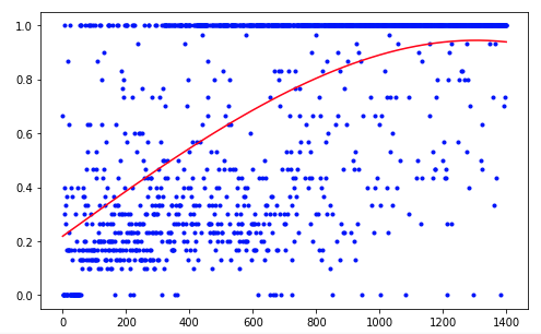
It took the agent 1,200 experiments to achieve about 95 percent of the result (the number of successful steps). And by the 50th experience, the Agent had learned to move the ball towards the goal (unsuccessful experiments disappear).

To improve the results, you can try to change the size of the network layers (LAYER_SIZE), the parameter of the discounting factor (GAMMA) or the rate of decrease in the probability of choosing a random action (LAMBDA).

Our Agent has the simplest architecture - DQN (Deep Q-Network). On such a simple task it is enough to get an acceptable result.

Using, for example, the DDQN (Double DQN) architecture should provide smoother, more accurate learning. And the RDQN network (Recurrent DQN) will be able to trace the patterns of the environment change over time, which will give the opportunity to get rid of the ball speed parameter, reducing the number of input network parameters.

You can also expand our simulation by adding the ball's variable mass or the angle of its motion.

But this is the next time.