Calculation of certain integrals: basic algorithms
This publication describes the simplest methods for calculating integrals of functions of one variable on an interval, also called quadrature formulas. Typically, these methods are implemented in standard math libraries, such as the GNU Scientific Library for C, SciPy for Python, and others. The publication aims to demonstrate how these methods work "under the hood", and to pay attention to some questions about the accuracy and performance of algorithms. I would also like to note the connection of quadrature formulas and methods for the numerical integration of ordinary differential equations, about which I want to write another publication.
Definition of the integral
Integral (Riemann function) f(x) on the segment [a;b] called the following limit:
intbaf(x)dx= lim Deltax to0 sumn−1i=0f( xii)(xi+1−xi), (1)
Where Deltax= max lbracexi+1−xi rbrace - the fineness of splitting, x0=a , xn=b , xii - an arbitrary number on the segment [xi;xi+1] .
If the integral of the function exists, then the limit value is the same regardless of the partition, if only it is quite small.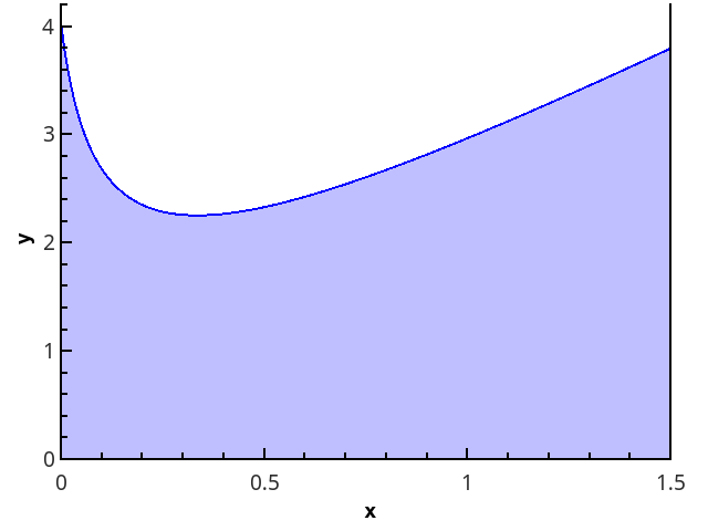
The geometrical definition is more obvious - the integral is equal to the area of a curvilinear trapezoid, bounded by the axis 0 x , the graph of the function and the straight lines x = a and x = b (the shaded area in the figure).
Quadrature formulas
The definition of integral (1) can be rewritten as
I= intbaf(x)dx approxIn=(b−a) sumn−1i=0wif( xii), (2)
Where wi - weight coefficients, the sum of which must be equal to 1, and the coefficients themselves - tend to zero with increasing number n points at which the function is calculated.
Expression (2) is the basis of all quadrature formulas (that is, formulas for the approximate calculation of the integral). The challenge is to select points lbrace xii rbrace and weight wi so that the sum on the right side approximates the required integral as precisely as possible.
Computational problem
Set function f(x) for which there is an algorithm for calculating values at any point of the segment [a;b] (meaning the points represented by a floating-point number — no Dirichlet functions there!).
Required to find the approximate value of the integral intbaf(x)dx .
Solutions will be implemented in Python 3.6.
The integral method is used to test the methods. int3/20 left[2x+ frac1 sqrtx+1/16 right]dx=17/4 .
Piece-constant approximation
The ideally simplest quadrature formulas arise from the use of the expression (1) "in the forehead":
In= sumn−1i=0f( xii)(xi+1−xi)
Since from the method of splitting a segment of dots lbracexi rbrace and point selection lbrace xii rbrace the value of the limit does not depend, then we will select them so that they are conveniently calculated - for example, we take the partitioning uniform, and for the points of calculation of the function we consider the options: 1) xii=xi ; 2) xii=xi+1 ; 3) xii=(xi+xi+1)/2 .
We obtain the methods of left rectangles, right rectangles and rectangles with a midpoint, respectively.
def _rectangle_rule(func, a, b, nseg, frac): """ .""" dx = 1.0 * (b - a) / nseg sum = 0.0 xstart = a + frac * dx # 0 <= frac <= 1 , # , # dx for i in range(npoints): sum += func(xstart + i * dx) return sum * dx def left_rectangle_rule(func, a, b, nseg): """ """ return _rectangle_rule(func, a, b, nseg, 0.0) def right_rectangle_rule(func, a, b, nseg): """ """ return _rectangle_rule(func, a, b, npoints, 1.0) def midpoint_rectangle_rule(func, a, b, nseg): """ """ return _rectangle_rule(func, a, b, nseg, 0.5) To analyze the performance of quadrature formulas, we construct a graph of the error in the coordinates “the number of points - the difference between the numerical result and the exact one”.
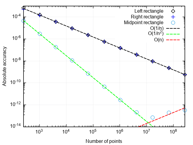
What can be noticed:
- The formula with a midpoint is much more accurate than with the right or left points.
- The error of a formula with a midpoint drops faster than the other two
- With a very fine partition, the error of the formula with the midpoint begins to increase
The first two points are related to the fact that the formula of rectangles with a midpoint has the second order of approximation, i.e. |In−I|=O(1/n2) , and the formulas of the right and left rectangles are the first order, i.e. |In−I|=O(1/n) .
The increase in the error during the grinding of the integration step is associated with the increase in the rounding error in the summation of a large number of terms. This error grows like |In−I|=O(1/n) that does not allow to achieve machine accuracy when integrated.
Conclusion: the methods of rectangles with right and left points have low accuracy, which also slowly grows with the refinement of the partition. Therefore, they only make sense for demonstration purposes. The method of rectangles with a midpoint has a higher approximation order, which gives it chances to be used in real applications (more on this below).
Piecewise linear approximation
The next logical step is to approximate an integrable function on each of the sub-segments by a linear function, which gives the quadrature trapezium formula:
In= sumn−1i=0 fracf(xi)+f(xi+1)2(xi+1−xi) (3)
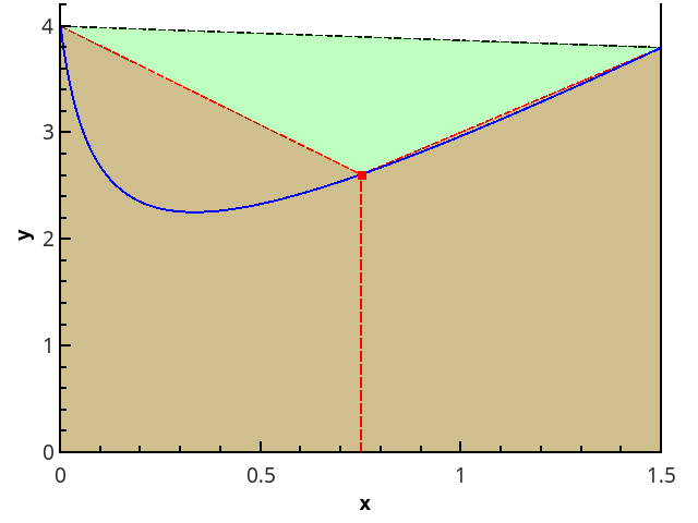
Illustration of the trapezoid method for n = 1 and n = 2.
In the case of a uniform grid, the lengths of all segments of the partition are equal, and the formula has the form
In=h left( fracf(a)+f(b)2+ sumn−1i=1f(a+ih) right), h= fracban (3a)
def trapezoid_rule(func, a, b, nseg): """ nseg - , [a;b]""" dx = 1.0 * (b - a) / nseg sum = 0.5 * (func(a) + func(b)) for i in range(1, nseg): sum += func(a + i * dx) return sum * dx By plotting the error from the number of split points, we see that the trapezoid method also has a second order of approximation and generally gives results that are slightly different from the middle point rectangle method (hereinafter, it is just the rectangle method).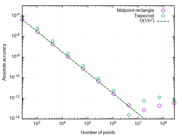
Accuracy control
Setting the number of split points as an input parameter is not very practical, since it is usually required to calculate the integral not with a given partition density, but with a given error. If the integrand function is known in advance, then it is possible to estimate the error in advance and choose such an integration step so that the specified accuracy is certainly achieved. But this is rarely the case in practice (and in general, is it not easier with a known function in advance and the integral itself to be tabulated in advance?), Therefore, a procedure is necessary to automatically adjust the step to a given error.
How to implement it? One of the simple methods for estimating an error — the Runge rule — the difference in the values of the integrals calculated over n and 2 n points, gives an estimate of the error: Delta2n approx|I2n−In| . The trapezoid method is more convenient for doubling the fineness of a partition than the method of rectangles with a central point. When calculating by the trapezoid method, to double the number of points, we need new values of the function only in the middle of the segments of the previous partition, i.e. The previous approximation of the integral can be used to calculate the following.
The method of rectangles does not require to calculate the function values at the ends of the segment. This means that it can be used for functions that have integrable singularities at the edges of a segment (for example, sin x / x or x -1/2 from 0 to 1). Therefore, the extrapolation method shown below will work in the same way for the rectangle method. The only difference from the trapezoidal method is that by decreasing the step, the result of previous calculations is doubled, but the number of points can be tripled , and then the previous value of the integral can also be used to calculate the new one. Formulas for extrapolation in this case must be adjusted to a different ratio of integration steps.
From here we get the following code for the trapezoid method with accuracy control:
def trapezoid_rule(func, a, b, rtol = 1e-8, nseg0 = 1): """ rtol - nseg0 - """ nseg = nseg0 old_ans = 0.0 dx = 1.0 * (b - a) / nseg ans = 0.5 * (func(a) + func(b)) for i in range(1, nseg): ans += func(a + i * dx) ans *= dx err_est = max(1, abs(ans)) while (err_est > abs(rtol * ans)): old_ans = ans ans = 0.5 * (ans + midpoint_rectangle_rule(func, a, b, nseg)) # # nseg *= 2 err_est = abs(ans - old_ans) return ans With this approach, the integrand will not be calculated several times at one point, and all calculated values are used for the final result.
But is it possible to achieve higher accuracy with the same amount of function calculations? It turns out that it is possible, there are formulas that work more precisely than the trapezoid method on the same grid.
Piecewise parabolic approximation
The next step is to approximate the function with elements of parabolas. This requires that the number of segments of the partition is even, then parabolas can be drawn through triples of points with abscissas {( x 0 = a , x 1 , x 2 ), ( x 2 , x 3 , x 4 ), ..., ( x n -2 , x n -1 , x n = b )}.
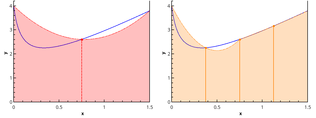
Illustration of the piecewise parabolic approximation at 3 and 5 points ( n = 2 and n = 3).
Approaching the integral of the function on each of the segments [ x k ; x k +2 ] integral of a parabolic approximation on this segment and considering the points evenly distributed ( x k +1 = x k + h ), we obtain the Simpson formula :
ISimps,n= sumn/2−1i=0 frach3[f(x2i)+4f(x2i+1)+f(x2i+2)]== frach3[f(a)+4f(a+h)+2f(a+2h)+...+4f(bh)+f(b)] (4)
Formula (4) directly yields the "naive" implementation of the Simpson method:
def simpson_rule(func, a, b, nseg): """ nseg - , [a;b]""" if nseg%2 = 1: nseg += 1 dx = 1.0 * (b - a) / nseg sum = (func(a) + 4 * func(a + dx) + func(b)) for i in range(1, nseg / 2): sum += 2 * func(a + (2 * i) * dx) + 4 * func(a + (2 * i + 1) * dx) return sum * dx / 3 To estimate the error, you can use the same calculation of the integral with steps h and h / 2 - but bad luck, when calculating the integral with a smaller step, you will have to discard the result of the previous calculation, although half of the new calculations of the function will be at the same points as before.
Fortunately, you can avoid wasting computer time by implementing the Simpson method in a more ingenious way. Looking closely, we note that the integral according to the Simpson formula can be represented through two integrals using the trapezoid formula with different steps. This is most clearly seen in the basic case of approximation of the integral over three points (a,f0), (a+h,f1), (a+2h,f2) :
ISimps,2= frach3(f0+4f1+f2)= frac43h left( fracf0+f12+ fracf1+f22 right)− frac13 cdot2h fracf0+f22== frac4Itrap,2−Itrap,13
Thus, if you implement the step reduction procedure in half and store the last two trapezoid calculations, the Simpson method with accuracy control is implemented more efficiently.
class Quadrature: """ """ __sum = 0.0 __nseg = 1 # __ncalls = 0 # def __restart(func, x0, x1, nseg0, reset_calls = True): """ . """ if reset_calls: Quadrature.__ncalls = 0 Quadrature.__nseg = nseg0 # nseg0 Quadrature.__sum = 0.5 * (func(x0) + func(x1)) dx = 1.0 * (x1 - x0) / nseg0 for i in range(1, nseg0): Quadrature.__sum += func(x0 + i * dx) Quadrature.__ncalls += 1 + nseg0 return Quadrature.__sum * dx def __double_nseg(func, x0, x1): """ . """ nseg = Quadrature.__nseg dx = (x1 - x0) / nseg x = x0 + 0.5 * dx i = 0 AddedSum = 0.0 for i in range(nseg): AddedSum += func(x + i * dx) Quadrature.__sum += AddedSum Quadrature.__nseg *= 2 Quadrature.__ncalls += nseg return Quadrature.__sum * 0.5 * dx def trapezoid(func, x0, x1, rtol = 1e-10, nseg0 = 1): """ . rtol - , nseg0 - """ ans = Quadrature.__restart(func, x0, x1, nseg0) old_ans = 0.0 err_est = max(1, abs(ans)) while (err_est > abs(rtol * ans)): old_ans = ans ans = Quadrature.__double_nseg(func, x0, x1) err_est = abs(old_ans - ans) print("Total function calls: " + str(Quadrature.__ncalls)) return ans def simpson(func, x0, x1, rtol = 1.0e-10, nseg0 = 1): """ . rtol - , nseg0 - """ old_trapez_sum = Quadrature.__restart(func, x0, x1, nseg0) new_trapez_sum = Quadrature.__double_nseg(func, x0, x1) ans = (4 * new_trapez_sum - old_trapez_sum) / 3 old_ans = 0.0 err_est = max(1, abs(ans)) while (err_est > abs(rtol * ans)): old_ans = ans old_trapez_sum = new_trapez_sum new_trapez_sum = Quadrature.__double_nseg(func, x0, x1) ans = (4 * new_trapez_sum - old_trapez_sum) / 3 err_est = abs(old_ans - ans) print("Total function calls: " + str(Quadrature.__ncalls)) return ans Compare the efficiency of the trapezoid method and parabolas:
>>> import math >>> Quadrature.trapezoid(lambda x: 2 * x + 1 / math.sqrt(x + 1 / 16), 0, 1.5, rtol=1e-9) Total function calls: 65537 4.250000001385811 >>> Quadrature.simpson(lambda x: 2 * x + 1 / math.sqrt(x + 1 / 16), 0, 1.5, rtol=1e-9) Total function calls: 2049 4.2500000000490985 As you can see, with both methods, the answer can be obtained with sufficiently high accuracy, but the number of calls to the integrand is strikingly different - a higher order method is 32 times more efficient!
By plotting the integration error versus the number of steps, it can be verified that the order of approximation of the Simpson formula is four, i.e. numerical integration error |ISimps,n−I|=O(1/n4) (and the integrals of cubic polynomials with the help of this formula are calculated to within rounding errors for any even n > 0!).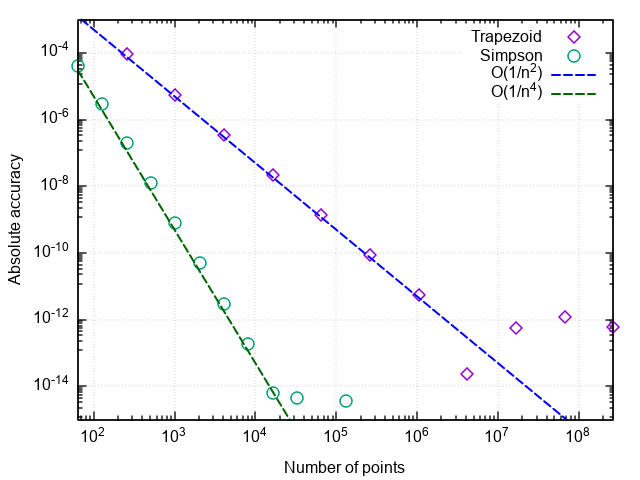
Hence, there is such an increase in efficiency compared to the simple trapezoidal formula.
What's next?
The further logic of improving the accuracy of quadrature formulas, in general, is understandable - if the function continues to be approximated by higher-order polynomials, then the integral of these polynomials will more closely approximate the integral of the original function. This approach is called the construction of Newton-Cotes quadrature formulas . Formulas are known up to the 8th order of approximation, but the alternating terms appear higher among the weighting factors w i in (2), and formulas lose their stability in the calculations.
Let's try to go some other way. The error of the quadrature formula is represented as a series in powers of the integration step h . A remarkable property of the trapezoidal method (and rectangles with a midpoint!) Is that for it this series consists only of even degrees:
Itrap,n[f,a,b]= intbaf(x)dx+C2h2+C4h4+C6h6+..., h= fracban (5)
Richardson extrapolation is based on finding successive approximations to this decomposition: instead of approximating the integrand function by a polynomial, the calculated approximations of the integral I(h) a polynomial approximation is constructed, which at h = 0 should give the best approximation to the true value of the integral.
The decomposition of the integration error in even powers of the partitioning step sharply accelerates the convergence of extrapolation, since for approximation of order 2 n you need only n values of the integral by the trapezoid method.
If we assume that each subsequent term is less than the previous one, then we can successively exclude the degrees h , having integral approximations calculated with different steps. Since the above implementation makes it easy to split the split in half, it is convenient to consider formulas for steps h and h / 2.
Itrap,n−I approxC2h2; Itrap,2n−I approxC2 left( frach2 right)2
It is easy to show that the elimination of the highest error term of the trapezoid formula will give a simpson formula:
I=Itrap,2n−C2 left( frach2 right)2+O(h4) approxItrap,2n− fracItrap,2n−Itrap,n1−22=ISimps,2n
Repeating a similar procedure for the Simpson formula, we get:
ISimps,2n−I approxC4 left( frach2 right)4; ISimps,n−I approxC4h4
I=ISimps,2n−C4 left( frach2 right)4+O(h6) approxISimps,2n− fracISimps,2n−ISimps,n1−24
If to continue, the following table appears:
| 2nd order | 4th order | 6 order | ... |
|---|---|---|---|
| I 0,0 | |||
| I 1,0 | I 1,1 | ||
| I 2,0 | I 2,1 | I 2,2 | |
| ... | ... | ... |
The first column contains the integrals calculated by the trapezoid method. When going from the top row down, the split of the segment becomes twice smaller, and when going from the left column to the right, the order of approximation of the integral increases (ie, the Simpson integrals in the second column, etc.).
The elements of the table, as can be derived from the decomposition (5), are related by the recurrence relation:
Ii,j=Ii,j−1− fracIi,j−1−Ii−1,j−11− left( frachijhi right)2=Ii,j−1− fracIi,j−1−Ii−1,j−11−22j (6)
The error of approximation of the integral can be estimated from the difference of formulas of different orders in one line, i.e.
Deltai,j approxIi,j−Ii,j−1
The use of Richardson extrapolation along with the integration of the trapezoid method is called the Romberg method . If the Simpson method takes into account the two previous values using the trapezoid method, the Romberg method uses all the values calculated by the trapezoid method earlier to obtain a more accurate estimate of the integral.
An additional method is added to the quadrature class.
class Quadrature: """ """ __sum = 0.0 __nseg = 1 # __ncalls = 0 # def __restart(func, x0, x1, nseg0, reset_calls = True): """ . """ if reset_calls: Quadrature.__ncalls = 0 Quadrature.__nseg = nseg0 # nseg0 Quadrature.__sum = 0.5 * (func(x0) + func(x1)) dx = 1.0 * (x1 - x0) / nseg0 for i in range(1, nseg0): Quadrature.__sum += func(x0 + i * dx) Quadrature.__ncalls += 1 + nseg0 return Quadrature.__sum * dx def __double_nseg(func, x0, x1): """ . """ nseg = Quadrature.__nseg dx = (x1 - x0) / nseg x = x0 + 0.5 * dx i = 0 AddedSum = 0.0 for i in range(nseg): AddedSum += func(x + i * dx) Quadrature.__sum += AddedSum Quadrature.__nseg *= 2 Quadrature.__ncalls += nseg return Quadrature.__sum * 0.5 * dx def romberg(func, x0, x1, rtol = 1e-10, nseg0 = 1, maxcol = 5, reset_calls = True): """ nseg0 - maxcol - """ # Itable = [[Quadrature.__restart(func, x0, x1, nseg0, reset_calls)]] i = 0 maxcol = max(0, maxcol) ans = Itable[i][i] error_est = max(1, abs(ans)) while (error_est > abs(rtol * ans)): old_ans = ans i += 1 d = 4.0 ans_col = min(i, maxcol) Itable.append([Quadrature.__double_nseg(func, x0, x1)] * (ans_col + 1)) for j in range(0, ans_col): diff = Itable[i][j] - Itable[i - 1][j] Itable[i][j + 1] = Itable[i][j] + diff / (d - 1.0) d *= 4.0 ans = Itable[i][ans_col] if (maxcol <= 1): # error_est = abs(ans - Itable[i - 1][-1]) elif (i > maxcol): error_est = abs(ans - Itable[i][min(i - maxcol - 1, maxcol - 1)]) else: error_est = abs(ans - Itable[i - 1][i - 1]) print("Total function calls: " + str(Quadrature.__ncalls)) return ans Check how the high order approximation works:
>>> Quadrature.romberg(lambda x: 2 * x + 1 / math.sqrt(x + 1/16), 0, 1.5, rtol=1e-9, maxcol = 0) # Total function calls: 65537 4.250000001385811 >>> Quadrature.romberg(lambda x: 2 * x + 1 / math.sqrt(x + 1/16), 0, 1.5, rtol=1e-9, maxcol = 1) # Total function calls: 2049 4.2500000000490985 >>> Quadrature.romberg(lambda x: 2 * x + 1 / math.sqrt(x + 1/16), 0, 1.5, rtol=1e-9, maxcol = 4) Total function calls: 257 4.250000001644076 We are convinced that, compared with the parabola method, the number of calls to the integrand has decreased by another 8 times. With a further increase in the required accuracy, the advantages of the Romberg method are even more pronounced: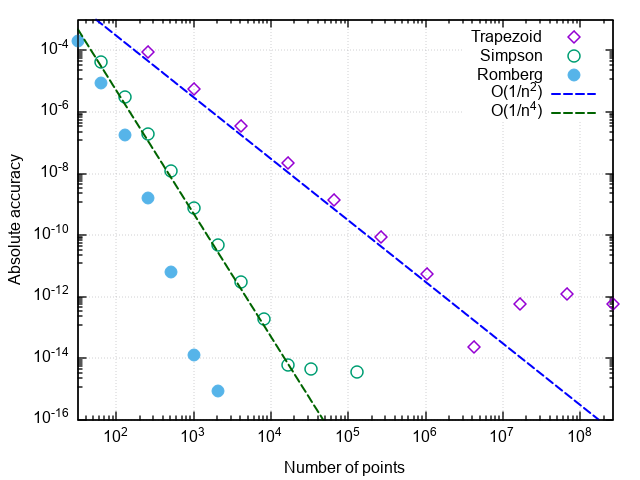
Some notes
Remark 1. The number of function calls in these problems characterizes the number of summations in the calculation of the integral. Reducing the number of computations of the integrand not only saves computational resources (although with a more optimized implementation, this is also the case), it also reduces the effect of round-off errors on the result. So, when trying to calculate the test function integral, the trapezoid method freezes when trying to achieve a relative accuracy of 5 × 10 -15 , a parabola method - at the desired accuracy of 2 × 10 -16 (which is the limit for doubles), and the Romberg method does the calculation test integral up to machine precision (with an error in the low bit). That is, not only the integration accuracy is increased for a given number of function calls, but also the maximum attainable accuracy of the integral calculation.
Remark 2. If the method converges when specifying a certain accuracy, this does not mean that the calculated value of the integral has the same accuracy. First of all, this applies to cases where the specified error is close to machine accuracy.
Remark 3. Although the Romberg method for a number of functions works in an almost magical way, it assumes that the integrand has bounded higher-order derivatives. This means that for functions with kinks or gaps, it may turn out to be worse than simple methods. For example, we integrate f ( x ) = | x |:
>>> Quadrature.trapezoid(abs, -1, 3, rtol=1e-5) Total function calls: 9 5.0 >>> Quadrature.simpson(abs, -1, 3, rtol=1e-5) Total function calls: 17 5.0 >>> Quadrature.romberg(abs, -1, 3, rtol=1e-5, maxcol = 2) Total function calls: 17 5.0 >>> Quadrature.romberg(abs, -1, 3, rtol=1e-5, maxcol = 3) Total function calls: 33 5.0 >>> Quadrature.romberg(abs, -1, 3, rtol=1e-5, maxcol = 4) Total function calls: 33 5.000001383269357 Remark 4. It may seem that the higher the order of approximation, the better. In fact, it is better to limit the number of columns of the Romberg table at level 4-6. To understand this, look at the formula (6). The second term is the difference of two consecutive elements of the j –1th column divided by about 4 j . Since in the j –1st column there are approximations of the integral of order 2 j , then the difference itself has order (1 / n i ) 2 j ~ 4 - ij . C division takes ~ 4 - ( i +1) j ~ 4 - j 2 . Those. when j ~ 7, the second term in (6) loses its accuracy after reducing the orders when adding floating-point numbers, and an increase in the approximation order can lead to an accumulation of rounding error.
Remark 5. Those interested can apply the described methods for finding the integral int10 sqrtx sinxdx and its equivalent int102t2 sint2dt . As they say, feel the difference.
Conclusion
A description and implementation of the basic methods of numerical integration of functions on a uniform grid is presented. It is demonstrated how using a simple modification to obtain, on the basis of the trapezoid method, a class of quadrature formulas using the Romberg method, which significantly accelerates the convergence of numerical integration. The method works well for integrating "normal" functions, i.e. weakly varying on the segment of integration, having no singularities on the edges of the segment (see Remark 5), fast oscillations, etc.
( [3] — C++).
Literature
- .. , .. . . .: . 1989.
- J. Stoer, R. Bulirsch. Introduction to Numerical Analysis: Second Edition. Springer-Verlag New York. 1993.
- WH Press, SA Teukolsky, WT Vetterling, BP Flannery. Numerical Recipes: Third Edition. Cambridge University Press. 2007
')
Source: https://habr.com/ru/post/420867/
All Articles