AI, practical course. The basic model of recognition of emotions in images

In this article, we will build a basic model of a convolutional neural network that is capable of recognizing emotions in images. Recognition of emotions in our case is a binary classification problem, the goal of which is to divide images into positive and negative.

All code, documents in notebook format and other materials, including the Dockerfile, can be found here .

Data

The first step in almost all machine learning tasks is to understand the data. Let's do that.
')

Dataset structure

Raw data can be downloaded here (in the Baseline.ipynb document, all actions in this section are performed automatically). The original data is in the archive format Zip *. Unpack it and examine the structure of the received files.



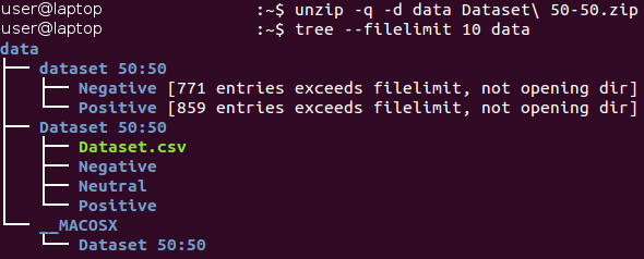
All images are stored inside the “dataset 50:50” directory and are distributed between its two subdirectories, whose name corresponds to their class — Negative and Positive. Note that the task is slightly unbalanced - 53 percent of the images are positive, and only 47 percent are negative. Typically, the data in classification tasks are considered unbalanced if the number of examples in different classes varies greatly. There are a number of ways to work with unbalanced data - for example, downsampling, resampling, changing data weights, etc. In our case, the imbalance is insignificant and should not drastically affect the learning process. It is only necessary to remember that the naive classifier, which always gives out a positive value, will provide an accuracy value of about 53 percent for this data set.

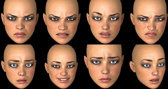
Let's look at several images of each class.

Negative







Positive







At first glance, images from different classes are actually different from each other. However, let's conduct a more in-depth study and try to find bad examples - similar images belonging to different classes.

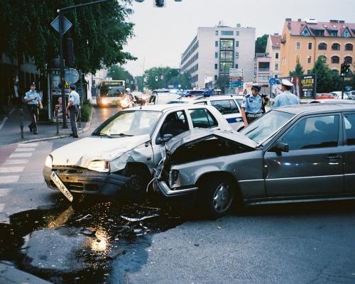
For example, we have about 90 images of snakes marked as negative and about 40 very similar images of snakes marked as positive.

Positive snake image



Negative Snake Image



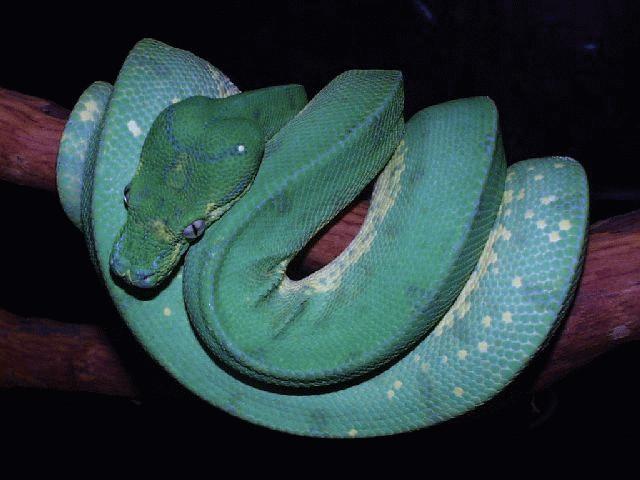
The same duality occurs with spiders (130 negative and 20 positive images), naked people (15 negative and 45 positive images), and some other classes. It seems that the labeling of images was performed by different people, and their perception of the same image may differ. Therefore, the marking contains its inherent inconsistency. These two images of snakes are almost identical, with different experts attributed them to different classes. Thus, it can be concluded that it is hardly possible to ensure 100% accuracy when working with this task due to its nature. We believe that a more realistic estimate of accuracy will be 80 percent — this value is based on the proportion of similar images found in various classes during the preliminary visual inspection.

Separation of the training / verification process

We always strive to create the best possible model. However, what is the meaning we put into this concept? There are many different criteria for this, such as: quality, lead time (learning + getting output) and memory consumption. Some of them can be easily and objectively measured (for example, time and amount of memory), while others (quality) are much more difficult to determine. For example, your model can demonstrate 100 percent accuracy when learning with examples that have been used to do this many times, but fail when working with new examples. This problem is called overfitting and is one of the most important in machine learning. There is also an under-fit problem: in this case, the model cannot learn from the data presented and demonstrates poor predictions even when using a fixed training data set.

To solve the problem of overfitting, the so-called technique of holding a part of the samples is used . Its main idea is to split the source data into two parts:

• A training set , which usually makes up most of the data set and is used to train the model.
• The test set is usually a small part of the source data, which is divided into two parts before performing all the training procedures. This set is not used at all in training and is considered as new examples for testing the model after completion of training.

Using this method, we can observe how well our model generalizes (that is, it works with previously unknown examples).

This article will use a 4/1 aspect ratio for the training and test sets. Another technique we use is the so-called stratification . This term means splitting each class independently of all other classes. This approach allows you to maintain the same balance between the size of the classes in the training and test sets. Stratification implicitly uses the assumption that the distribution of examples does not change when the source data is changed and remains the same when using new examples.



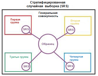
We illustrate the concept of stratification with a simple example. Suppose that we have four data groups / classes with the corresponding number of objects in them: children (5), teenagers (10), adults (80) and elderly people (5); see the picture on the right (from Wikipedia ). Now we need to split this data into two sets of samples in a ratio of 3/2. When using stratification of examples, objects will be selected independently from each group: 2 objects from a group of children, 4 objects from a group of teenagers, 32 objects from a group of adults, and 2 objects from a group of elderly people. The new data set contains 40 objects, which is exactly 2/5 of the original data. At the same time, the balance between the classes in the new data set corresponds to their balance in the original data.

All the above actions are implemented in a single function called prepare_data ; This function can be found in the utils.py Python file. This function loads data, breaks it up into training and test sets using a fixed random number (for later playback), and then distributes the data appropriately between directories on the hard disk for later use.

Pretreatment and augmentation

In a previous article, preprocessing actions and possible reasons for their use in the form of augmentation data were described. Convolutional neural networks are quite complex models, and their training requires large amounts of data. In our case there are only 1600 examples - this, of course, is not enough.

Therefore, we want to expand the set of data used by augmentation data . In accordance with the information provided in the article on data preprocessing, the Keras * library provides the ability to augment data on the fly when reading it from a hard disk. This can be done through the ImageDataGenerator class.



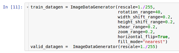
Here are two instances of generators. The first copy is intended for training and uses many random transformations - such as rotation, shift, convolution, scaling and horizontal rotation - while reading data from the disk and transferring it to the model. As a result, the model receives already transformed examples, and each example obtained by the model is unique due to the random nature of this transformation. The second copy is intended for verification, and it only zooms the images. The training and verification generators have only one common transformation - the zoom. To ensure the computational stability of the model, it is necessary to use the range [0; 1] instead of [0; 255].

Model architecture

After studying and preparing the initial data, the model creation stage follows. Since a small amount of data is available to us, we are going to build a relatively simple model in order to be able to train it accordingly and eliminate the oversampling situation. Let's try the VGG style architecture , however we use fewer layers and filters.





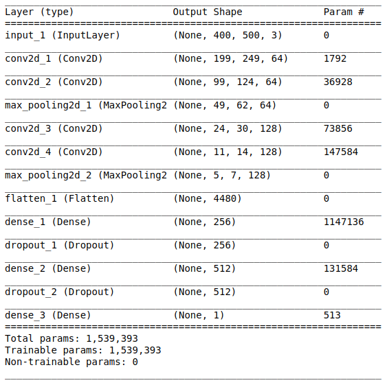
The network architecture consists of the following parts:
[Convolutional layer + convolutional layer + selection of the maximum value] × 2
The first part contains two superimposed convolutional layers with 64 filters (with size 3 and step 2) and a layer for selecting the maximum value (with size 2 and step 2), located after them. This part is also commonly referred to as a feature extraction unit , since filters effectively extract significant features from the input data (see the article Overview of convolutional neural networks to classify images for more information).

Alignment

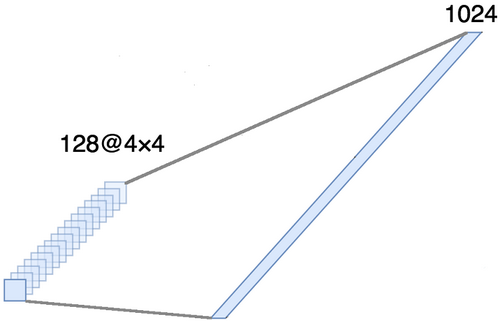
This part is mandatory, since at the output of the convolutional part four-dimensional tensors are obtained (examples, height, width and channels). However, for the usual fully connected layer, we need a two-dimensional tensor (examples, signs) as input data. Therefore, it is necessary to align the tensor around the last three axes in order to combine them into one axis. In fact, this means that we consider each point in each feature map as a separate property and align them into one vector. The figure below shows an example of a 4 × 4 image with 128 channels, which is aligned into one long vector with a length of 1024 elements.



[Full connected layer + elimination method] × 2

Before you is the classification part of the network. It takes an aligned representation of the attributes of the images and tries to classify them in the best possible way. This part of the network consists of two superimposed blocks consisting of a fully connected layer and an exclusion method . We have already met with fully connected layers - usually these are layers with fully connected connectivity. But what is the “exception method”? The exclusion method is a regularization technique that helps prevent oversubset. One of the possible signs of overfitting is the extremely different values ​​of the weighting factors (the orders of the corresponding quantities). There are many ways to solve this problem, including weight reduction and the method of elimination. The idea of ​​the exclusion method is to disable random neurons during training (the list of disabled neurons must be updated after each packet / epoch of training). This greatly hinders the obtaining of completely different values ​​for the weights, thus regularizing the network.



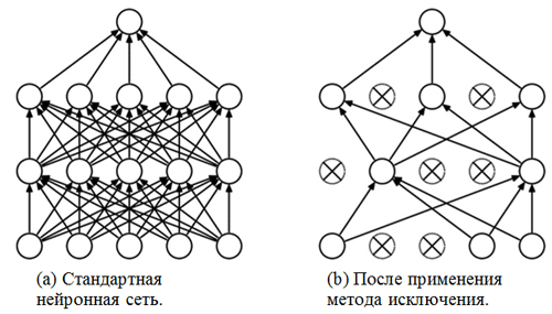
An example of the use of the elimination method (picture taken from the article The elimination method: an easy way to prevent oversampling in neural networks ):

Sigmoid module

The output layer must correspond to the formulation of the problem. In this case, we are dealing with a binary classification problem, so we need one output neuron with a sigmoid activation function, which estimates the probability P of belonging to class number 1 (in our case, these will be positive images). Then the probability of belonging to class number 0 (negative images) can easily be calculated as 1 - P.

Settings and learning options

We chose the model architecture and specified it using the Keras library for the Python language. In addition, before you start learning the model, you must compile it.



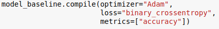
At the compilation stage, the model is configured for training. It is necessary to specify three main parameters:

• Optimizer . In this case, we use the Adam * default optimizer, which is a type of stochastic gradient descent algorithm with momentum and adaptive learning rate (for more information, see S. Ruder blog entry Overview of Gradient Descent Optimization Algorithms ).
• Loss function Our task is a binary classification problem, so it would be appropriate to use binary cross entropy as a loss function.
• Metrics . This is an optional argument by which you can specify additional metrics to track during the training procedure. In this case, we need to track accuracy along with the objective function.

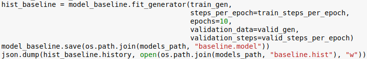
Now we are ready to learn the model. Note that the learning procedure is performed using generators initialized in the previous section.

The number of epochs is another hyperparameter that can be customized. Here we simply assign it a value of 10. We also want to save the model and the learning history in order to be able to load it later.

Evaluation

Now let's see how well our model works. First of all, consider the change in metrics in the learning process.



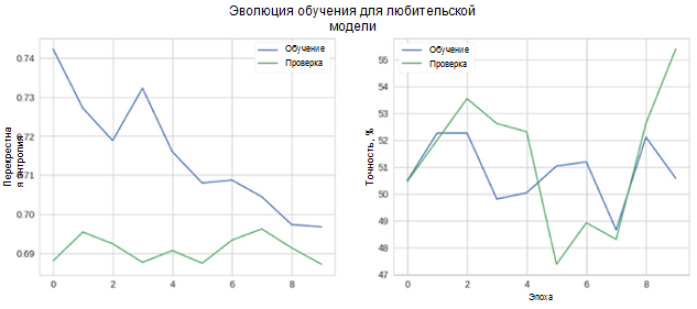
In the figure, it can be seen that cross-validation entropy and accuracy do not decrease over time. Moreover, the accuracy metric for training and test sets simply fluctuates around the value of the random classifier. The total accuracy for the test set is 55 percent, which is only slightly better than a random estimate.

Let's look at how model predictions are distributed between classes. For this purpose, it is necessary to create and visualize an inaccuracy matrix using the appropriate function from the Sklearn * package for the Python language.
Each cell in the inaccuracy matrix has its own name:

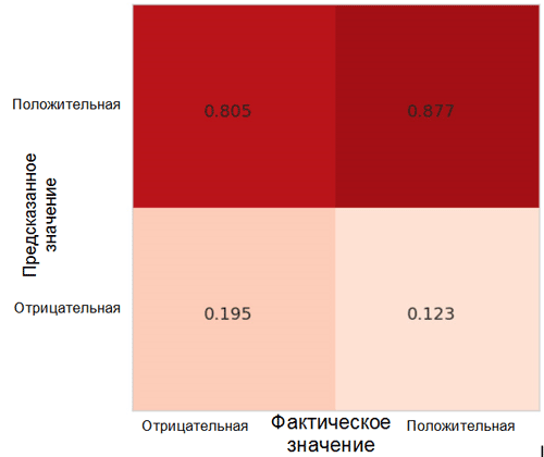
• True Positive Rate = TPR (upper right cell) represents the proportion of positive examples (class 1, that is, positive emotions in our case), which are correctly classified as positive.
• False Positive Rate = FPR (lower right cell) represents the proportion of positive examples that are incorrectly classified as negative (class 0, that is, negative emotions).
• True Negative Rate = TNR (lower left cell) represents the proportion of negative examples that are correctly classified as negative.
• False Negative Rate = FNR (upper left cell) represents the proportion of negative examples that are classified in the wrong way as positive.

In our case, both the TPR and FPR values ​​are close to 1. This means that almost all the objects were classified as positive. Thus, our model is not far removed from the naive base model with constant predictions of a larger class size (in our case, these are positive images).

Another interesting metric that is interesting to observe is the receiver’s performance curve (ROC curve) and the area under this curve (ROC AUC). A formal definition of these concepts can be found here . In a nutshell, the ROC curve shows how well the binary classifier works.

The classifier of our convolutional neural network has a sigmoid module as an output, which assigns the probability of example to class 1. Now suppose that our classifier shows good performance and assigns low probability values ​​for examples of class 0 (green histogram in the figure below) and high probability values ​​for examples class 1 (histogram blue).



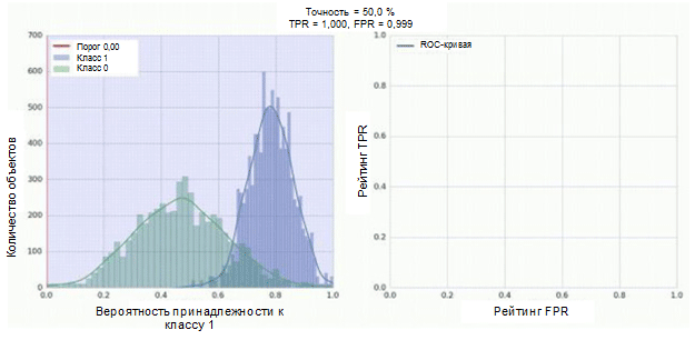
The ROC curve shows how the TPR depends on the FPR when moving the classification threshold from 0 to 1 (right figure, top). For a better understanding of the concept of a threshold, remember that we have the probability of belonging to class 1 for each example. However, probability is not yet a class label. Therefore, it should be compared with the threshold to determine which class the example belongs to. For example, if the threshold value is 1, then all examples should be classified as belonging to class 0, since the probability value cannot be more than 1, and the values ​​of the FPR and TPR indicators will be equal to 0 (since none of the samples are classified as positive ). This situation corresponds to the leftmost point on the ROC curve. On the other side of the curve, there is a point at which the threshold value is 0: this means that all samples are classified as belonging to class 1, and the values ​​of both TPR and FPR are 1. Intermediate points reflect the behavior of the TPR / FPR dependency when the threshold value changes.

The diagonal line on the graph corresponds to a random classifier. The better our classifier works, the closer its curve is to the left upper point of the graph. Thus, the objective indicator of the quality of the classifier is the area under the ROC curve (ROC AUC). The value of this indicator should be as close as possible to 1. AUC value of 0.5, corresponds to a random classifier.

The AUC in our model (see figure above) is 0.57, which is not the best result.



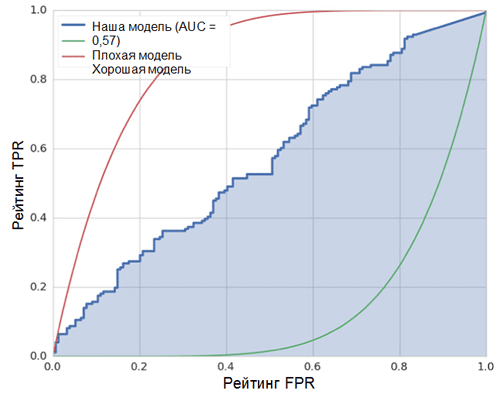
All these metrics indicate that the resulting model is only slightly better than the random classifier. There are several reasons for this, the main ones are described below:

• A very small amount of data for training, insufficient to highlight the characteristic features of images. Even data augmentation could not help in this case.
• A relatively complex convolutional neural network model (compared to other machine learning models) with a large number of parameters.

Conclusion

In this article, we created a simple convolutional neural network model for recognizing emotions in images. At the same time, at the training stage, a number of methods were used for augmentation of data, the model was also evaluated using a set of metrics such as: accuracy, ROC-curve, ROC AUC and inaccuracy matrix. The model showed results, only slightly better than random ones. The reason for this is the lack of available data.