Diarization based on GMM-UBM model and MAP adaptation algorithm
Hi, Habr. I would like to talk about one of the approaches in solving the problem of diarization of announcers and show how this method can be implemented in python. In order not to scare away the reader, I will not give complex mathematical formulas (partly because I myself am “not a real welder”), but I will try to explain everything in simple language and tell everything so that the developer has never come across machine learning.
In preparing to write this article, I chose between two presentation options: for those who are already familiar with Data Science and those who simply program well. In the end, I chose the second option, deciding that this would be a good demonstration of the capabilities of DS.
As Wikipedia tells us, diarization is the process of dividing an incoming audio stream into homogeneous segments according to the audio stream belonging to one or another speaker. In other words, the record should be divided into pieces and numbered: here in these places one person says, but in these places another. From the point of view of machine learning, this kind of tasks belong to the class of education without a teacher and are called clustering. About what clustering methods exist, for example , you can read here or here , but I will only seed those that will be useful to us - this is a Gaussian Mixture Model and Spectral Clustering. But about them a bit later.
Let's start from the beginning.
Generally speaking, besides R, the python language is the main one in solving Data Science problems, and if you have not tried programming on it, I highly recommend it, because python allows you to do many things elegantly, literally in a few lines (by the way, there are even such a meme).
')
There are two separately developing branches of python - versions 2 and 3. In my examples, I used version 3.6, but if you like, you can easily port them to version 2.7. It is convenient to deploy any of these branches together with the Anaconda installer, having installed which you immediately get an interactive shell for development - IPython.
In addition to the development environment itself, additional libraries will be needed: librosa (for working with audio and extracting features), webrtcvad (for segmentation), and pickle (for writing trained models to a file). All of them are installed by a simple team in Anaconda Prompt
We begin by extracting the traits — the data the machine learning models will work with. In principle, the audio signal itself is already data, namely an ordered array of sound amplitude values, to which is added a header containing the number of channels, the sampling frequency, and other information. But we will not be able to analyze this data directly, since they do not contain such things, looking at which, our model can say - aha, these pieces belong to the same person.
There are several approaches to feature extraction in speech processing tasks. One of them is to obtain chalk-frequency cepstral coefficients (Mel Frequency Cepstral Coefficients). We have already written about them here, so I’ll just slightly remind you.
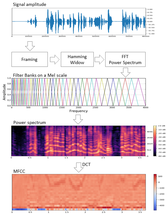
The original signal is cut into frames with a length of 16-40 ms. Next, applying the Hamming window to the frame, we make a fast Fourier transform and obtain the power spectral density. Then, a special “comb” of filters located evenly along the chalk scale makes a chalk spectrogram, to which a discrete cosine transform (DCT), a widely used data compression algorithm, is applied. The coefficients obtained in this way are a kind of compressed frame characteristic, and since the filters we used were located in the chalk scale, the coefficients carry more information in the human ear’s perception range. Typically, 13 to 25 MFCC per frame is used. Since, in addition to the spectrum itself, the personality of the voice is shaped by speed and acceleration, MFCC is combined with the first and second derivatives.
In general, MFCC is the most common way of working with speech, but besides them there are other signs - LPC (Linear Predictive Coding) and PLP (Perceptual Linear Prediction), and sometimes you can also find LFCC, where instead of chalk-scale linear is used.
Let's see how to extract MFCC in python.
As you can see, this is really done in just a few lines. We now turn to the first clustering algorithm.
The model of a mixture of Gaussian distributions assumes that our data are a mixture of multidimensional Gaussian distributions with certain parameters.
If you wish, you can easily find both a detailed description of the model and how the EM algorithm that teaches this model works, but I promised not to cause melancholy with complex formulas and therefore I will show beautiful examples from this article.
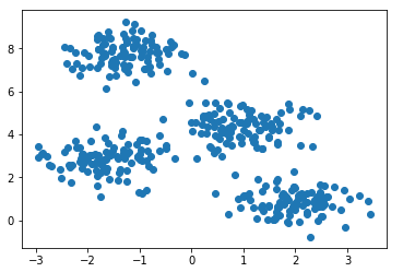
Generate four clusters and draw them.
We will create a model, train it on our data and again draw points, but already taking into account the predicted model of belonging to clusters.
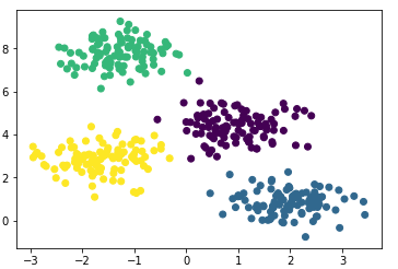
The model coped well with artificial data. In principle, by adjusting the number of components of the mixture and the type of the covariance matrix (the number of degrees of freedom of Gaussians), one can describe rather complex data.

So, we know how to do parameterization of data and know how to train a model of a mixture of Gaussian distributions. Now one could try to do head-on clustering - teaching GMM on the MFCC extracted from the dialogue. And, probably, in some ideal spherical-vacuum dialogue, in which each speaker will fit into his Gaussian, we will get a good result. It is clear that in reality this will never happen. In fact, with the help of GMM, it is not the dialogue that is being modeled, but each person in the dialogue — that is, they represent that each speaker’s voice in the extracted features is described by his own set of Gaussians.
Summing up, we slowly get to the main topic.
Traditionally, the diarization process consists of three consecutive blocks - voice detection (Voice Activity Detection), segmentation and clustering (there are models in which the last two steps are combined, see LIA E-HMM ).
In the first step, speech is separated from various kinds of noise. The VAD algorithm determines whether a piece of audio filed on it is a speech, or if, for example, a siren sounds or someone sneezes. It is clear that in order for such an algorithm to be of high quality, training with a teacher is necessary. And this in turn means that it is necessary to mark up the data - in other words, to create a database with records of speech and all sorts of noise. We will act lazily - take ready VAD , which does not work perfectly, but for the beginning we have enough.
The second block cuts data into segments with one active speaker. The classical approach in this regard is the algorithm for determining the change of speaker based on the Bayesian information criterion - BIC . The essence of this method is as follows: a sliding window traverses audio recordings and at each point of the passage answers the question: “How are the data in this place better described - in one distribution or two?”. To answer this question, the parameter is calculated. , based on the sign of which the decision is made to change the speaker. The problem is that this method will not work very well in case of a frequent change of announcer, and even in the presence of noise (which is very characteristic for recording a telephone conversation).
In conditions when the speakers do not interrupt each other, and their voices do not overlap each other, the VAD, which we will use, more or less copes with the task of segmentation, so the first two steps will look like this.
In fact, people will certainly talk at the same time. Moreover, VAD in some places blundered, due to the fact that the recording is not live, but is a gluing, in which pauses are cut. You can try to repeat the cutting into segments, increasing the aggressiveness of VAD from 2 to 3.
Now we have separate segments, and we decided that we would be using GMM to model each speaker. We will extract the signs from the segment and use this data to train the model. We will do so on each segment and the resulting models are comparable. It is justified to expect that models trained in segments belonging to the same person will be somehow similar. But here we are faced with the following problem, extracting signs from an audio file of 1 sec length with a sampling frequency of 8000 Hz with a window size of 10 ms, we get a set of 800 MFCC vectors. On such data, our model will not be able to learn, because it is negligible. Even if it is not one second, but ten, the data will still not be enough. And here the Universal Background Model (UBM) comes to the rescue, it is also called the speaker-independent. The idea is as follows. We will train GMM on a large sample of data (in our case, this is a complete recording of the interview) and we will get the acoustic model of a generalized announcer (this will be our UBM). And then, using a special adaptation algorithm (about it a little lower), we will “fit” this model to the characteristics extracted from each segment. This approach is widely used not only for diarization, but also in voice recognition systems. To recognize a person by voice, you first need to train a model on it and, without UBM, you would need to have several hours to record this person’s speech.
From each adapted GMM, we extract a vector of shear coefficients. (he is a median or a mat. wait, if you will) and, based on the data on these vectors from all segments, we will do the clustering (below it will be clear why the shift vector is the one).
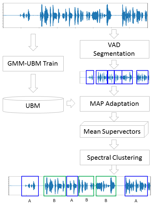
The method by which we will customize UBM for each segment is called Maximum A-Posteriori Adaptation. In general, the algorithm is as follows. First, the posterior probability on the adaptation data and sufficient statistics for the weight, median and variance of each Gaussian are calculated. Then the statistics obtained are combined with the UBM parameters and the parameters of the adapted model are obtained. In our case, we will only adapt the median, without affecting the other parameters. Despite the fact that I promised not to delve into mathematics, I’ll give you three formulas, because MAP adaptation is the key point in this article.
Here - a posteriori probability - sufficient statistics for , - median of the adapted model, - coefficient of adaptation, - Compliance factor.
If all this seems rubbish and causes despondency - do not despair. In fact, to understand the operation of the algorithm, it is not necessary to delve into these formulas, its work can be easily demonstrated by the following example:
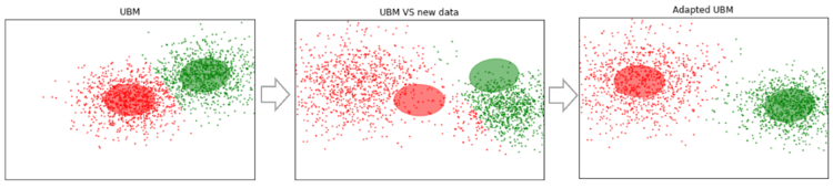
Suppose we have some fairly large data, and we have trained on them UBM (left figure, UBM is a two-component mixture of Gaussian distributions). There are new data that do not fit into our model (figure in the middle). Using this algorithm, we will shift the Gaussian centers so that they fit into the new data (figure on the right). Applying this algorithm on experimental data, we would expect that on segments with the same speaker Gaussians will shift in the same direction, thus forming clusters. That is why for clustering segments we will use the data about the shift .
So let's do a MAP adaptation for each segment. (For reference: besides MAP Adaptation, the MLLR - Maximum Likelihood Linear Regression method and some modifications are widely used. Also try to combine these two methods.)
Now that for each segment we have data on , we finally go to the final step.
Spectral clustering is briefly described in the article, the link to which I gave at the very beginning. The algorithm builds a complete graph, where the vertices are our data, and the edges between them are a measure of similarity. In voice recognition tasks, the cosine metric is used as such a measure, since it takes into account the angle between the vectors, ignoring their magnitude (which does not carry information about the speaker). By constructing a graph, the eigenvectors of the Kirchhoff matrix (which is essentially a representation of the graph obtained) are calculated and then some standard clustering method is used, for example, the k-means method. All this keeps within two lines of code.
The described algorithm was tested with various parameters:
As a result, the parameters remained subjectively optimal: MFCC 13, GMM covariance_type = 'full' n_components = 16.
Unfortunately, I didn’t have the patience (I started writing this article more than a month ago) in order to mark up the received segments and calculate the DER (Diariztion Error Rate). Subjectively, I rate the work of the algorithm as “in principle not bad, but far from ideal”. By clustering on vectors derived from the first hundred segments (with one MAP pass), and then highlighting those where the interviewer speaks (the girl, she speaks much less guest there), clustering produces a list that is 100% hit. In this case, there are segments where both speakers are present (for example, 14), but this can already be blamed on the VAD error. Moreover, such segments begin to count with an increase in the number of MAP passes. An important point. Interviews with which we worked - more or less “clean”. If various musical inserts, noises and other non-speech things are added, clustering starts to limp. Therefore, plans to try to train your own VAD (because webrtcvad, for example, does not separate music from speech).
Due to the fact that I initially worked with a telephone conversation, I did not need to estimate the number of announcers. But the number of announcers is not always predetermined, even if it is an interview. For example, in this interview in the middle there is an announcement superimposed on the music, and voiced by an additional two people. Therefore, it would be interesting to try the method for estimating the number of announcers indicated in the first article in the section of the list of references (based on the analysis of the eigenvalues of the normalized Laplace matrix).
In addition to the materials located on the links in the text and Jupyter laptops, the following sources were used to prepare this article:
I also add some diarrhea projects:
All the code is laid out on the githaba . For convenience, I made several Jupyter laptops with a demonstration of individual items - MFCC, GMM, MAP Adaptation and Diarization. In the latter is the main process. Also in the repository are pickle files with some pre-trained models and the interview itself.
In preparing to write this article, I chose between two presentation options: for those who are already familiar with Data Science and those who simply program well. In the end, I chose the second option, deciding that this would be a good demonstration of the capabilities of DS.
Formulation of the problem
As Wikipedia tells us, diarization is the process of dividing an incoming audio stream into homogeneous segments according to the audio stream belonging to one or another speaker. In other words, the record should be divided into pieces and numbered: here in these places one person says, but in these places another. From the point of view of machine learning, this kind of tasks belong to the class of education without a teacher and are called clustering. About what clustering methods exist, for example , you can read here or here , but I will only seed those that will be useful to us - this is a Gaussian Mixture Model and Spectral Clustering. But about them a bit later.
Let's start from the beginning.
Environment preparation
Spoiler
I was not sure whether to leave this section - I didn’t want to turn the article into a very tutorial. But in the end left. Who does not need, he will miss, and for those who will do everything from scratch, this step will facilitate the start.
Generally speaking, besides R, the python language is the main one in solving Data Science problems, and if you have not tried programming on it, I highly recommend it, because python allows you to do many things elegantly, literally in a few lines (by the way, there are even such a meme).
')
There are two separately developing branches of python - versions 2 and 3. In my examples, I used version 3.6, but if you like, you can easily port them to version 2.7. It is convenient to deploy any of these branches together with the Anaconda installer, having installed which you immediately get an interactive shell for development - IPython.
In addition to the development environment itself, additional libraries will be needed: librosa (for working with audio and extracting features), webrtcvad (for segmentation), and pickle (for writing trained models to a file). All of them are installed by a simple team in Anaconda Prompt
pip install [library] Feature Extraction
We begin by extracting the traits — the data the machine learning models will work with. In principle, the audio signal itself is already data, namely an ordered array of sound amplitude values, to which is added a header containing the number of channels, the sampling frequency, and other information. But we will not be able to analyze this data directly, since they do not contain such things, looking at which, our model can say - aha, these pieces belong to the same person.
There are several approaches to feature extraction in speech processing tasks. One of them is to obtain chalk-frequency cepstral coefficients (Mel Frequency Cepstral Coefficients). We have already written about them here, so I’ll just slightly remind you.
The original signal is cut into frames with a length of 16-40 ms. Next, applying the Hamming window to the frame, we make a fast Fourier transform and obtain the power spectral density. Then, a special “comb” of filters located evenly along the chalk scale makes a chalk spectrogram, to which a discrete cosine transform (DCT), a widely used data compression algorithm, is applied. The coefficients obtained in this way are a kind of compressed frame characteristic, and since the filters we used were located in the chalk scale, the coefficients carry more information in the human ear’s perception range. Typically, 13 to 25 MFCC per frame is used. Since, in addition to the spectrum itself, the personality of the voice is shaped by speed and acceleration, MFCC is combined with the first and second derivatives.
In general, MFCC is the most common way of working with speech, but besides them there are other signs - LPC (Linear Predictive Coding) and PLP (Perceptual Linear Prediction), and sometimes you can also find LFCC, where instead of chalk-scale linear is used.
Let's see how to extract MFCC in python.
import numpy as np import librosa mfcc=librosa.feature.mfcc(y=y, sr=sr, hop_length=int(hop_seconds*sr), n_fft=int(window_seconds*sr), n_mfcc=n_mfcc) mfcc_delta=librosa.feature.delta(mfcc) mfcc_delta2=librosa.feature.delta(mfcc, order=2) stacked=np.vstack((mfcc, mfcc_delta, mfcc_delta2)) features=stacked.T #librosa MFCC , . As you can see, this is really done in just a few lines. We now turn to the first clustering algorithm.
Gaussian Mixture Model
The model of a mixture of Gaussian distributions assumes that our data are a mixture of multidimensional Gaussian distributions with certain parameters.
If you wish, you can easily find both a detailed description of the model and how the EM algorithm that teaches this model works, but I promised not to cause melancholy with complex formulas and therefore I will show beautiful examples from this article.
Generate four clusters and draw them.
from sklearn.datasets.samples_generator import make_blobs X, y_true=make_blobs(n_samples=400, centers=4, cluster_std=0.60, random_state=0) plt.scatter(X[:, 0], X[:, 1]); We will create a model, train it on our data and again draw points, but already taking into account the predicted model of belonging to clusters.
from sklearn.mixture import GaussianMixture gmm = GaussianMixture(n_components=4) gmm.fit(X) labels=gmm.predict(X) plt.scatter(X[:, 0], X[:, 1], c=labels, s=40, cmap='viridis'); The model coped well with artificial data. In principle, by adjusting the number of components of the mixture and the type of the covariance matrix (the number of degrees of freedom of Gaussians), one can describe rather complex data.
So, we know how to do parameterization of data and know how to train a model of a mixture of Gaussian distributions. Now one could try to do head-on clustering - teaching GMM on the MFCC extracted from the dialogue. And, probably, in some ideal spherical-vacuum dialogue, in which each speaker will fit into his Gaussian, we will get a good result. It is clear that in reality this will never happen. In fact, with the help of GMM, it is not the dialogue that is being modeled, but each person in the dialogue — that is, they represent that each speaker’s voice in the extracted features is described by his own set of Gaussians.
Summing up, we slowly get to the main topic.
Segmentation
Traditionally, the diarization process consists of three consecutive blocks - voice detection (Voice Activity Detection), segmentation and clustering (there are models in which the last two steps are combined, see LIA E-HMM ).
In the first step, speech is separated from various kinds of noise. The VAD algorithm determines whether a piece of audio filed on it is a speech, or if, for example, a siren sounds or someone sneezes. It is clear that in order for such an algorithm to be of high quality, training with a teacher is necessary. And this in turn means that it is necessary to mark up the data - in other words, to create a database with records of speech and all sorts of noise. We will act lazily - take ready VAD , which does not work perfectly, but for the beginning we have enough.
The second block cuts data into segments with one active speaker. The classical approach in this regard is the algorithm for determining the change of speaker based on the Bayesian information criterion - BIC . The essence of this method is as follows: a sliding window traverses audio recordings and at each point of the passage answers the question: “How are the data in this place better described - in one distribution or two?”. To answer this question, the parameter is calculated. , based on the sign of which the decision is made to change the speaker. The problem is that this method will not work very well in case of a frequent change of announcer, and even in the presence of noise (which is very characteristic for recording a telephone conversation).
A little explanation
In the original, I worked with telephone call center recordings with an average duration of about 4 minutes. For obvious reasons, I cannot post these recordings, so for the demonstration I took a recording of an interview from one radio station. In the case of a long interview, this method would probably give an acceptable result, but it did not work on my data.
In conditions when the speakers do not interrupt each other, and their voices do not overlap each other, the VAD, which we will use, more or less copes with the task of segmentation, so the first two steps will look like this.
# y_, sr = librosa.load('data/2018-08-26-beseda-1616.mp3', sr=SR) # pre-emphasis: pre_emphasis = 0.97 y = np.append(y[0], y[1:] - pre_emphasis * y[:-1]) # webrtcvad vad = webrtcvad.Vad(2) # VAD audio = np.int16(y/np.max(np.abs(y)) * 32767) frames = frame_generator(10, audio, sr) frames = list(frames) segments = vad_collector(sr, 50, 200, vad, frames) if not os.path.exists('data/chunks'): os.makedirs('data/chunks') for i, segment in enumerate(segments): chunk_name = 'data/chunks/chunk-%003d.wav' % (i,) # vad , write_wave(chunk_name, segment[0: len(segment)-int(100*sr/1000)], sr) In fact, people will certainly talk at the same time. Moreover, VAD in some places blundered, due to the fact that the recording is not live, but is a gluing, in which pauses are cut. You can try to repeat the cutting into segments, increasing the aggressiveness of VAD from 2 to 3.
GMM-UBM
Now we have separate segments, and we decided that we would be using GMM to model each speaker. We will extract the signs from the segment and use this data to train the model. We will do so on each segment and the resulting models are comparable. It is justified to expect that models trained in segments belonging to the same person will be somehow similar. But here we are faced with the following problem, extracting signs from an audio file of 1 sec length with a sampling frequency of 8000 Hz with a window size of 10 ms, we get a set of 800 MFCC vectors. On such data, our model will not be able to learn, because it is negligible. Even if it is not one second, but ten, the data will still not be enough. And here the Universal Background Model (UBM) comes to the rescue, it is also called the speaker-independent. The idea is as follows. We will train GMM on a large sample of data (in our case, this is a complete recording of the interview) and we will get the acoustic model of a generalized announcer (this will be our UBM). And then, using a special adaptation algorithm (about it a little lower), we will “fit” this model to the characteristics extracted from each segment. This approach is widely used not only for diarization, but also in voice recognition systems. To recognize a person by voice, you first need to train a model on it and, without UBM, you would need to have several hours to record this person’s speech.
From each adapted GMM, we extract a vector of shear coefficients. (he is a median or a mat. wait, if you will) and, based on the data on these vectors from all segments, we will do the clustering (below it will be clear why the shift vector is the one).
MAP Adaptation
The method by which we will customize UBM for each segment is called Maximum A-Posteriori Adaptation. In general, the algorithm is as follows. First, the posterior probability on the adaptation data and sufficient statistics for the weight, median and variance of each Gaussian are calculated. Then the statistics obtained are combined with the UBM parameters and the parameters of the adapted model are obtained. In our case, we will only adapt the median, without affecting the other parameters. Despite the fact that I promised not to delve into mathematics, I’ll give you three formulas, because MAP adaptation is the key point in this article.
Here - a posteriori probability - sufficient statistics for , - median of the adapted model, - coefficient of adaptation, - Compliance factor.
If all this seems rubbish and causes despondency - do not despair. In fact, to understand the operation of the algorithm, it is not necessary to delve into these formulas, its work can be easily demonstrated by the following example:
Suppose we have some fairly large data, and we have trained on them UBM (left figure, UBM is a two-component mixture of Gaussian distributions). There are new data that do not fit into our model (figure in the middle). Using this algorithm, we will shift the Gaussian centers so that they fit into the new data (figure on the right). Applying this algorithm on experimental data, we would expect that on segments with the same speaker Gaussians will shift in the same direction, thus forming clusters. That is why for clustering segments we will use the data about the shift .
So let's do a MAP adaptation for each segment. (For reference: besides MAP Adaptation, the MLLR - Maximum Likelihood Linear Regression method and some modifications are widely used. Also try to combine these two methods.)
SV = [] # chunk-000 chunk-100 for i in range(101): clear_output(wait=True) fname='data/chunks/chunk-%003d.wav' % (i,) print('UBM MAP adaptation for {0}'.format(fname)) y_, sr_ = librosa.load(fname, sr=None) f_ = extract_features(y_, sr_, window=N_FFT, hop=HOP_LENGTH, n_mfcc=N_MFCC) f_ = preprocessing.scale(f_) gmm = copy.deepcopy(ubm) gmm = map_adaptation(gmm, f_, max_iterations=1, relevance_factor=16) sv = gmm.means_.flatten() # sv = preprocessing.scale(sv) SV.append(sv) SV = np.array(SV) clear_output() print(SV.shape) Now that for each segment we have data on , we finally go to the final step.
Spectral clustering
Spectral clustering is briefly described in the article, the link to which I gave at the very beginning. The algorithm builds a complete graph, where the vertices are our data, and the edges between them are a measure of similarity. In voice recognition tasks, the cosine metric is used as such a measure, since it takes into account the angle between the vectors, ignoring their magnitude (which does not carry information about the speaker). By constructing a graph, the eigenvectors of the Kirchhoff matrix (which is essentially a representation of the graph obtained) are calculated and then some standard clustering method is used, for example, the k-means method. All this keeps within two lines of code.
N_CLUSTERS = 2 sc = SpectralClustering(n_clusters=N_CLUSTERS, affinity='cosine') labels = sc.fit_predict(SV) # , . [2,1,1,0,2] labels = rearrange(labels, N_CLUSTERS) # [0,1,1,2,0] print(labels) # , , 1 - . print([i for i, x in enumerate(labels) if x == 1]) Conclusions and future plans
The described algorithm was tested with various parameters:
- Number of MFCC: 7, 13, 20
- MFCC in combination with LPC
- Type and number of mixtures in GMM: full [8, 16, 32], diag [8, 16, 32, 64, 256]
- UBM adaptation methods: MAP (with covariance_type = 'full') and MLLR (with covariance_type = 'diag')
As a result, the parameters remained subjectively optimal: MFCC 13, GMM covariance_type = 'full' n_components = 16.
Unfortunately, I didn’t have the patience (I started writing this article more than a month ago) in order to mark up the received segments and calculate the DER (Diariztion Error Rate). Subjectively, I rate the work of the algorithm as “in principle not bad, but far from ideal”. By clustering on vectors derived from the first hundred segments (with one MAP pass), and then highlighting those where the interviewer speaks (the girl, she speaks much less guest there), clustering produces a list that is 100% hit. In this case, there are segments where both speakers are present (for example, 14), but this can already be blamed on the VAD error. Moreover, such segments begin to count with an increase in the number of MAP passes. An important point. Interviews with which we worked - more or less “clean”. If various musical inserts, noises and other non-speech things are added, clustering starts to limp. Therefore, plans to try to train your own VAD (because webrtcvad, for example, does not separate music from speech).
Due to the fact that I initially worked with a telephone conversation, I did not need to estimate the number of announcers. But the number of announcers is not always predetermined, even if it is an interview. For example, in this interview in the middle there is an announcement superimposed on the music, and voiced by an additional two people. Therefore, it would be interesting to try the method for estimating the number of announcers indicated in the first article in the section of the list of references (based on the analysis of the eigenvalues of the normalized Laplace matrix).
Bibliography
In addition to the materials located on the links in the text and Jupyter laptops, the following sources were used to prepare this article:
- Speaker Diarization using GMM Supervector and Advanced Reduction Algorithms. Nurit spingarn
- Feature Extraction Methods LPC, PLP and MFCC In Speech Recognition. Namrata dave
- MAP estimation for mulivariate gaussian mixture of observations of markov chains. Jean-Luc Gauvain and Chin-Hui Lee
- On Spectral Clustering Analysis and an algorithm. Andrew Y. Ng, Michael I. Jordan, Yair Weiss
- Speaker recognition using YOHO database. Alexandre Majetniak
I also add some diarrhea projects:
- Sidekit and diarization extension for s4d . Python library for speech. Unfortunately, the documentation leaves much to be desired.
- Bob and its different parts like bob.bio , bob.learn.em is a python library for signal processing and working with biometric data. Windows is not supported.
- LIUM is a turnkey solution written in Java.
All the code is laid out on the githaba . For convenience, I made several Jupyter laptops with a demonstration of individual items - MFCC, GMM, MAP Adaptation and Diarization. In the latter is the main process. Also in the repository are pickle files with some pre-trained models and the interview itself.
Source: https://habr.com/ru/post/420515/
All Articles