Water rendering in screen space

My last task in technical graphics / rendering was finding a good solution for rendering water. In particular, the rendering of thin and fast moving water jets on the basis of particles. Last week I thought of good results, so I will write an article about it.

I don’t really like the approach of voxelized / marching cubes when rendering water (see, for example, rendering a fluid simulation in Blender). When the volume of water is on the same scale as the grid used for rendering, the movement is noticeably discrete. This problem can be solved by increasing the grid resolution, but for thin jets over relatively long distances in real time, this is simply impractical, because it greatly affects the execution time and the memory taken. (There is a precedent for using sparse voxel structures that improves the situation. But I'm not sure how well this works for dynamic systems. In addition, this is not the level of complexity I would like to work with.)

The first alternative I explored was meshes from Müller's Screen Space Meshes. They use rendering of water particles to the depth buffer, smoothing it, recognizing connected fragments of similar depth, and building a mesh from the result using marching squares. Today, this method has probably already become more applicable than in 2007 (since now we can create a mesh in the compute shader), but it is still associated with a greater level of complexity and cost than I would like.
')
In the end, I found Simon Green's presentation with GDC 2010 “Screen Space Fluid Rendering For Games”. It starts in the same way as Screen Space Meshes: from particle rendering to the depth buffer and its smoothing. But instead of building the mesh, the resulting buffer is used for shading and compositing the fluid in the main scene (by explicitly recording the depth.) I decided to implement just such a system.

Training

Several previous projects in Unity have taught me not to deal with the limitations of rendering the engine. Therefore, the fluid buffers are rendered by a second camera with a smaller depth of field, so that it is rendered in front of the main scene. Each fluid system exists on a separate rendering layer; the main chamber excludes a layer of water, and the second chamber renders only water. Both cameras are child elements of an empty object to ensure their mutual orientation.

This scheme means that I can render almost anything in the fluid layer, and it will look like I expect it. In the context of my demo scene, this means that several streams and splashes from subemitters can merge together. In addition, this will allow other water systems to be mixed in, for example, volumes based on height fields, which can then be rendered equally. (I haven't tested it yet.)

The source of water in my scene is a standard particle system. In fact, no fluid simulation is performed. This in turn means that the particles overlap each other in a not entirely physical way, but the end result looks acceptable in practice.

Fluid buffer rendering

The first step in this technique is the rendering of the base fluid buffer. This is an off-screen buffer that contains (at the current stage of my implementation) the following: the width of the fluid, the motion vector in the screen space, and the noise value. In addition, we render the depth buffer by explicitly writing the depth from the fragment shader to turn each quadrangle of the particle into a spherical (well, actually elliptical) “ball”.

The depth and width calculations are fairly simple:

frag_out o; float3 N; N.xy = i.uv*2.0 - 1.0; float r2 = dot(N.xy, N.xy); if (r2 > 1.0) discard; Nz = sqrt(1.0 - r2); float4 pixel_pos = float4(i.view_pos + N * i.size, 1.0); float4 clip_pos = mul(UNITY_MATRIX_P, pixel_pos); float depth = clip_pos.z / clip_pos.w; o.depth = depth; float thick = Nz * i.size * 2; 

(Of course, depth calculations can be simplified; we need only z and w from the clip position.)

A little later we will return to the fragment shader for the sake of motion vectors and noise.

The fun starts in the vertex shader, and it is here that I deviate from the Green technique. The goal of this project is to render high-speed water jets; it can be realized with the help of spherical particles, but to create a continuous jet will require a huge number of them. Instead, I will stretch the quadrangles of the particles based on their speed, which in turn stretches the depth balls, making them not spherical, but elliptical. (Because depth calculations are based on UVs that do not change, it all just works.)

Experienced Unity users may wonder why I simply do not use the built-in Stretched Billboard mode found in the Unity particle system. Stretched Billboard performs unconditional stretching along the velocity vector in the space of the world. In the general case, this is quite suitable, but it leads to a very noticeable problem when the velocity vector is co-directed with the forward vector of the camera (or very close to it). Billboard stretches the screen, which makes its two-dimensional nature very noticeable.

Instead, I use a camera-directed billboard and project the velocity vector onto the plane of the particle, using it to stretch the quad. If the velocity vector is perpendicular to the plane (sent to or away from the screen), then the particle remains unstretched and spherical, as it should, and when it is tilted, the particle stretches in that direction, which is what we need.

Leave a long explanation, here is a fairly simple function:

 float3 ComputeStretchedVertex(float3 p_world, float3 c_world, float3 vdir_world, float stretch_amount) { float3 center_offset = p_world - c_world; float3 stretch_offset = dot(center_offset, vdir_world) * vdir_world; return p_world + stretch_offset * lerp(0.25f, 3.0f, stretch_amount); } 

To calculate the motion vector of the screen space, we calculate two sets of vector positions:

 float3 vp1 = ComputeStretchedVertex( vertex_wp, center_wp, velocity_dir_w, rand); float3 vp0 = ComputeStretchedVertex( vertex_wp - velocity_w * unity_DeltaTime.x, center_wp - velocity_w * unity_DeltaTime.x, velocity_dir_w, rand); o.motion_0 = mul(_LastVP, float4(vp0, 1.0)); o.motion_1 = mul(_CurrVP, float4(vp1, 1.0)); 

Notice that since we compute the motion vectors in the main pass and not in the speed vectors pass, Unity does not provide us with a previous or undistorted current projection from view. To fix this, I added a simple script to the corresponding particle systems:

 public class ScreenspaceLiquidRenderer : MonoBehaviour { public Camera LiquidCamera; private ParticleSystemRenderer m_ParticleRenderer; private bool m_First; private Matrix4x4 m_PreviousVP; void Start() { m_ParticleRenderer = GetComponent(); m_First = true; } void OnWillRenderObject() { Matrix4x4 current_vp = LiquidCamera.nonJitteredProjectionMatrix * LiquidCamera.worldToCameraMatrix; if (m_First) { m_PreviousVP = current_vp; m_First = false; } m_ParticleRenderer.material.SetMatrix("_LastVP", GL.GetGPUProjectionMatrix(m_PreviousVP, true)); m_ParticleRenderer.material.SetMatrix("_CurrVP", GL.GetGPUProjectionMatrix(current_vp, true)); m_PreviousVP = current_vp; } } 

I cache the previous matrix manually, because Camera.previousViewProjectionMatrix gives incorrect results.

¯ \ _ (ツ) _ / ¯

(This method also violates rendering rendering; it may be wise to set global matrix constants in practice rather than using them for each material.)

Let's return to the fragment shader: we use the projected positions to calculate the motion vectors of the screen space:

 float3 hp0 = i.motion_0.xyz / i.motion_0.w; float3 hp1 = i.motion_1.xyz / i.motion_1.w; float2 vp0 = (hp0.xy + 1) / 2; float2 vp1 = (hp1.xy + 1) / 2; #if UNITY_UV_STARTS_AT_TOP vp0.y = 1.0 - vp0.y; vp1.y = 1.0 - vp1.y; #endif float2 vel = vp1 - vp0; 

(Motion vector calculations are almost unchanged from https://github.com/keijiro/ParticleMotionVector/blob/master/Assets/ParticleMotionVector/Shaders/Motion.cginc )

Finally, the last value in the fluid buffer is noise. I use a stable random number for each particle to select one of the four noises (packed in a single texture). It then scales to speed and unit minus particle size (therefore, fast and small particles are noisier). This noise value is used in the shading pass to distort the normals and add a layer of foam. Green's work uses three-channel white noise, but in a newer work (“Screen Space Fluid Rendering with Curvature Flow”) it is proposed to use Perlin noise. I use Voronoi noise / cellular noise with different scales:

Mixing problems (and workarounds)

And here the first problems of my implementation appear. To correctly calculate the thickness of the particles are mixed additively. Since mixing affects all outputs, this means that noise and motion vectors are also mixed additively. The additive noise suits us perfectly, but not the additive vectors, and if you leave them as they are, you get a disgusting time anti-aliasing (TAA) and motion blur. To solve this problem, when rendering the fluid buffer, I simply multiply the motion vectors by the thickness and divide by the total thickness in the shading passage. This gives us a weighted average motion vector for all overlapping particles; not exactly what we need (strange artifacts are created when crossing several jets), but quite acceptable.

The more difficult problem is depth; for the correct rendering of the depth buffer, we need to have both depth recording and depth checking being active at the same time. This can cause problems if the particles are not sorted (since the difference in rendering order can cause the output data of particles overlapped by others to be cut off). Therefore, we order the Unity particle system to sort the particles by depth, and then we cross our fingers and hope. that the systems will also be rendered in depth. We * will * have cases of imposing systems (for example, the intersection of two jets of particles) that are processed incorrectly, which will lead to a smaller thickness. But this does not happen very often, and does not greatly affect the appearance.

Most likely, the correct approach would be to completely separate rendering of the depth and color buffers; The cost for this will be rendering in two passes. It is worth studying this issue when setting up the system.

Depth smoothing

Finally, the most important thing in the technique of Green. We have rendered a bunch of spherical balls to the depth buffer, but in reality the water does not consist of “balls”. So now we take this approximation and blur it so that it looks more like a liquid surface.

The naive approach is to apply the Gaussian noise to the entire depth buffer. It creates strange results - smoothes distant points more strongly than close ones, and blurs the edges of the silhouettes. Instead, we can change the blur radius in depth, and use a two-sided blur to save edges.

Here there is only one problem: such changes make the blur inseparable. Shared blur can be performed in two passes: blur horizontally and then vertically. Unshared blur is performed in one pass. This distinction is important because the split blur scales linearly (O (w) + O (h)), and the non-separable scale quadratically (O (w * h)). Large-scale indivisible blur quickly becomes inapplicable in practice.

As adults, responsible developers, we can make an obvious move: close your eyes, pretend that two-way noise * is * separable, and still implement it with separate horizontal and vertical aisles.

Green, in his presentation, demonstrated that although this approach creates artifacts in the resulting result (especially during normal reconstruction), the shading phase hides them well. When working with narrower jets of water that I create, these artifacts are even less noticeable and do not really affect the result.

Shading

We finally finished working with the fluid buffer. We now turn to the second part of the effect: shading and compositing the main image.

Here we face a variety of Unity rendering constraints. I decided to light the water only with the light of the sun and skybox; supporting additional sources of illumination requires either several passes (it is wasteful!) or building a search structure for lighting on the GPU side (expensive and quite difficult). In addition, since Unity does not provide access to shadow maps, and directional lighting sources (directional lights) use screen space shadows (based on the depth buffer rendered by opaque geometry), we do not have access to information about shadows from the source of sunlight. You can attach a command buffer to the source of sunlight to create a shadow map of screen space specifically for water, but so far I have not done so.

The last stage of shading is controlled through a script, and uses a command buffer for sending draw calls. This is necessary because the motion vector texture (used for temporary anti-aliasing (TAA) and motion blur) cannot be used for direct rendering with Graphics.SetRenderTarget (). In the script attached to the main camera, we write the following:

 void Start() { //... m_QuadMesh = new Mesh(); m_QuadMesh.subMeshCount = 1; m_QuadMesh.vertices = new Vector3[] { new Vector3(0, 0, 0.1f), new Vector3(1, 0, 0.1f), new Vector3(1, 1, 0.1f), new Vector3(0, 1, 0.1f), }; m_QuadMesh.uv = new Vector2[] { new Vector2(0, 0), new Vector2(1, 0), new Vector2(1, 1), new Vector2(0, 1), }; m_QuadMesh.triangles = new int[] { 0, 1, 2, 0, 2, 3, }; m_QuadMesh.UploadMeshData(false); m_CommandBuffer = new CommandBuffer(); m_CommandBuffer.Clear(); m_CommandBuffer.SetProjectionMatrix( GL.GetGPUProjectionMatrix( Matrix4x4.Ortho(0, 1, 0, 1, -1, 100), false)); m_CommandBuffer.SetRenderTarget( BuiltinRenderTextureType.CameraTarget, BuiltinRenderTextureType.CameraTarget); m_CommandBuffer.DrawMesh( m_QuadMesh, Matrix4x4.identity, m_Mat, 0, m_Mat.FindPass("LIQUIDCOMPOSITE")); m_CommandBuffer.SetRenderTarget( BuiltinRenderTextureType.MotionVectors, BuiltinRenderTextureType.Depth); m_CommandBuffer.DrawMesh( m_QuadMesh, Matrix4x4.identity, m_Mat, 0, m_Mat.FindPass("MOTION")); } 

Color and motion vector buffers cannot be simultaneously rendered using MRT (multi render targets). I could not find out the reason. In addition, they require binding to different depth buffers. Fortunately, we are recording depth into both of these depth buffers, so re-projection of temporary anti-aliasing works fine (oh, this is the pleasure of working with the black box engine).

In each frame, we throw out the composite render from OnPostRender ():

 RenderTexture GenerateRefractionTexture() { RenderTexture result = RenderTexture.GetTemporary(m_MainCamera.activeTexture.descriptor); Graphics.Blit(m_MainCamera.activeTexture, result); return result; } void OnPostRender() { if (ScreenspaceLiquidCamera && ScreenspaceLiquidCamera.IsReady()) { RenderTexture refraction_texture = GenerateRefractionTexture(); m_Mat.SetTexture("_MainTex", ScreenspaceLiquidCamera.GetColorBuffer()); m_Mat.SetVector("_MainTex_TexelSize", ScreenspaceLiquidCamera.GetTexelSize()); m_Mat.SetTexture("_LiquidRefractTexture", refraction_texture); m_Mat.SetTexture("_MainDepth", ScreenspaceLiquidCamera.GetDepthBuffer()); m_Mat.SetMatrix("_DepthViewFromClip", ScreenspaceLiquidCamera.GetProjection().inverse); if (SunLight) { m_Mat.SetVector("_SunDir", transform.InverseTransformVector(-SunLight.transform.forward)); m_Mat.SetColor("_SunColor", SunLight.color * SunLight.intensity); } else { m_Mat.SetVector("_SunDir", transform.InverseTransformVector(new Vector3(0, 1, 0))); m_Mat.SetColor("_SunColor", Color.white); } m_Mat.SetTexture("_ReflectionProbe", ReflectionProbe.defaultTexture); m_Mat.SetVector("_ReflectionProbe_HDR", ReflectionProbe.defaultTextureHDRDecodeValues); Graphics.ExecuteCommandBuffer(m_CommandBuffer); RenderTexture.ReleaseTemporary(refraction_texture); } } 

And this is where CPU participation ends, only shaders come later.

Let's start with the passage of motion vectors. This is what the whole shader looks like:

 #include "UnityCG.cginc" sampler2D _MainDepth; sampler2D _MainTex; struct appdata { float4 vertex : POSITION; float2 uv : TEXCOORD0; }; struct v2f { float2 uv : TEXCOORD0; float4 vertex : SV_POSITION; }; v2f vert(appdata v) { v2f o; o.vertex = mul(UNITY_MATRIX_P, v.vertex); o.uv = v.uv; return o; } struct frag_out { float4 color : SV_Target; float depth : SV_Depth; }; frag_out frag(v2f i) { frag_out o; float4 fluid = tex2D(_MainTex, i.uv); if (fluid.a == 0) discard; o.depth = tex2D(_MainDepth, i.uv).r; float2 vel = fluid.gb / fluid.a; o.color = float4(vel, 0, 1); return o; } 

The speed in screen space is stored in the green and blue channel of the fluid buffer. Since rendering the buffer we scaled the speed by thickness, we again divide the total thickness (located in the alpha channel) to get a weighted average speed.

It is worth noting that when working with large volumes of water, another method of processing the velocity buffer may be required. As we render without blending, motion vectors for everything behind the water are lost, destroying the TAA and motion blur of these objects. When working with thin streams of water is not a problem, but can interfere when working with a pool or a lake, when we need TAA or motion blur objects to be clearly visible through the surface.

The main pass of shading is more interesting. Our first priority after masking with the help of the thickness of the liquid is to reconstruct the position and the normal of the viewing space (view space).

 float3 ViewPosition(float2 uv) { float clip_z = tex2D(_MainDepth, uv).r; float clip_x = uv.x * 2.0 - 1.0; float clip_y = 1.0 - uv.y * 2.0; float4 clip_p = float4(clip_x, clip_y, clip_z, 1.0); float4 view_p = mul(_DepthViewFromClip, clip_p); return (view_p.xyz / view_p.w); } float3 ReconstructNormal(float2 uv, float3 vp11) { float3 vp12 = ViewPosition(uv + _MainTex_TexelSize.xy * float2(0, 1)); float3 vp10 = ViewPosition(uv + _MainTex_TexelSize.xy * float2(0, -1)); float3 vp21 = ViewPosition(uv + _MainTex_TexelSize.xy * float2(1, 0)); float3 vp01 = ViewPosition(uv + _MainTex_TexelSize.xy * float2(-1, 0)); float3 dvpdx0 = vp11 - vp12; float3 dvpdx1 = vp10 - vp11; float3 dvpdy0 = vp11 - vp21; float3 dvpdy1 = vp01 - vp11; // Pick the closest float3 dvpdx = dot(dvpdx0, dvpdx0) > dot(dvpdx1, dvpdx1) ? dvpdx1 : dvpdx0; float3 dvpdy = dot(dvpdy0, dvpdy0) > dot(dvpdy1, dvpdy1) ? dvpdy1 : dvpdy0; return normalize(cross(dvpdy, dvpdx)); } 

This is a costly way of reconstructing the position of the viewing space: we take a position in the clip space and perform the inverse operation of the projection.

After we have obtained the method for reconstructing positions, with the normals everything is simpler: we calculate the position of the neighboring points in the depth buffer and build a tangent basis on them. To work with the edges of the silhouettes, we perform sampling in both directions and select the closest point in the view space for the reconstruction of the normal. This method works surprisingly well and causes problems only in the case of very thin objects.

This means that we perform five separate backward projection operations (for the current point and four adjacent ones) per pixel. There is a less expensive way, but this post is already too long, so I will leave it for later.

The resulting normals are:


I distort this computed normal with the help of the derivatives of the noise value from the fluid buffer scaled by the force parameter and normalized by splitting the jet thickness (for the same reason as for the speed):

 N.xy += NoiseDerivatives(i.uv, fluid.r) * (_NoiseStrength / fluid.a); N = normalize(N); 

We can finally proceed to the very shading.Water shading consists of three main parts: specular reflection, specular refraction and foam.

Reflection is a standard GGX, entirely taken from the standard Unity shader. (With one correction, the correct F0 equal to 2% is used for water.)

With refraction it is more and more interesting. For correct refraction, raytracing is required (or raymarching for an approximate result). Fortunately, refraction is less intuitive to the eye than reflection, and therefore incorrect results are not so noticeable. Therefore, we shift the UV sample for the refraction texture by x and y normals, scaled by thickness and force parameter:

 float aspect = _MainTex_TexelSize.y * _MainTex_TexelSize.z; float2 refract_uv = (i.grab_pos.xy + N.xy * float2(1, -aspect) * fluid.a * _RefractionMultiplier) / i.grab_pos.w; float4 refract_color = tex2D(_LiquidRefractTexture, refract_uv); 

(Note that correlation is used; it is optional — after all, this is just an approximation, but adding it is quite simple.)

This refracted light passes through the liquid, so part of it is absorbed:

 float3 water_color = _AbsorptionColor.rgb * _AbsorptionIntensity; refract_color.rgb *= exp(-water_color * fluid.a); 

Notice that _AbsorptionColor is defined in exactly the opposite way expected: the values ​​of each channel indicate the amount of light absorbed , not transmitted. Therefore, _AbsorptionColor with the value (1, 0, 0) does not give red, but turquoise (teal).

Reflection and refraction are mixed using Fresnel coefficients:

 float spec_blend = lerp(0.02, 1.0, pow(1.0 - ldoth, 5)); float4 clear_color = lerp(refract_color, spec, spec_blend); 

Up to this point, we played by the rules (mostly) and used physical shading.

He is quite good, but he has a problem with water. Its a bit hard to see:


To eliminate it, let's add some foam.

Foam appears when water is turbulent and air mixes with water to form bubbles. Such bubbles create all sorts of variations of reflection and refraction, which gives all the water a sense of diffused lighting. I will model this behavior with wrapped diffuse lighting:

 float3 foam_color = _SunColor * saturate((dot(N, L)*0.25f + 0.25f)); 

It is added to the final color using a special factor, depending on the noise of the fluid and a softened Fresnel coefficient:

 float foam_blend = saturate(fluid.r * _NoiseStrength) * lerp(0.05f, 0.5f, pow(1.0f - ndotv, 3)); clear_color.rgb += foam_color * saturate(foam_blend); 

Wrapped ambient lighting is normalized to conserve energy, so that it can be used as an approximation of scattering. The mixing of the foam color is more noticeable. It is quite a clear violation of the law of conservation of energy.

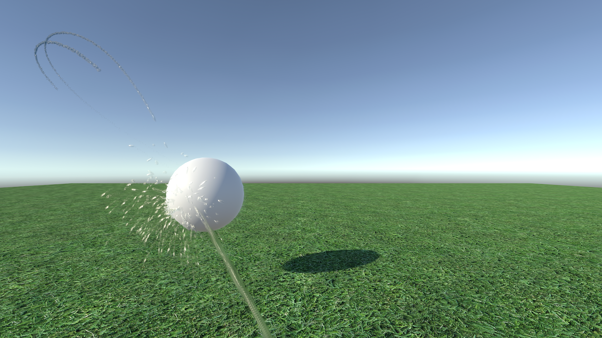
But in general, everything looks good and makes the jet more noticeable:

Further work and improvements

Much can be improved in the created system.

• Use multiple colors. Currently, the absorption is calculated only at the last shading stage and uses constant color and brightness for all the liquid on the screen. Supporting different colors is possible, but requires a second color buffer and solving the absorption integral for each particle in the rendering process of the basic fluid buffer. This could potentially be a costly operation.
• Full coverage. Having access to the lighting search structure on the GPU side (either built by hand or linked to the new Unity HD rendering pipeline), we can properly light the water with an arbitrary number of light sources and create the correct ambient lighting.
• Improved refraction. With the help of blurred mip-textures of the background texture, we can better simulate the refraction for rough surfaces. In practice, this is not very useful for small jets of fluid, but can be useful for large volumes.

If I had the opportunity, I would improve this system to a loss of pulse, but at the moment it can be called complete.