USE, RED, PgBouncer, its settings and monitoring

We started updating the monitoring service for PgBouncer in our service and decided to do a bit of combing. To make everything fit, we pulled the most famous monitoring performance methodologies: Brendan Gregg’s USE (Utilization, Saturation, Errors) and Tom Wilkie’s RED (Requests, Errors, Durations).

Under the cut, there is a story with graphs about how pgbouncer works, what configuration handles it has, and how to choose the right metrics for its monitoring using USE / RED.

First, about the methods themselves

Although these methods are quite well-known ( they were already on Habré, though not very detailed ), but not that they are widespread in practice.

USE

For each resource, follow recycling, saturation and errors.
Brendan gregg

Here, a resource is any individual physical component - CPU, disk, bus, etc. But not only - the performance of some software resources can also be considered by this method, in particular, virtual resources, such as containers / cgroups with limits, are also conveniently considered.

U - Recycling : either the percentage of time (from the observation interval) when the resource was occupied by useful work. Like, for example, CPU utilization or disk utilization, 90% means that 90% of the time was occupied with something useful) or, for resources such as memory, this is the percentage of memory used.

In any case, 100% recycling means that the resource can not be used more than now. And either the work will be stuck waiting for release / sent to the queue, or there will be errors. These two scenarios are covered by the corresponding two remaining USE metrics:

S - Saturation , it's saturation: a measure of the amount of "delayed" / queued work.

E - Errors : just count the number of failures. Errors / failures affect performance, but they may not be immediately noticeable due to rerai of fired operations or fault tolerance mechanisms with backup devices, etc.

RED

Tom Wilkie (now working at Grafana Labs) was frustrated by the USE methodology, or rather, by its poor applicability in some cases and inconsistencies in practice. How, for example, to measure the saturation of memory? Or how to measure errors in the system bus in practice?

Linux, it turns out, really sucks error counters.
T. Wilkie

In short, to monitor performance and the behavior of microservices, he suggested another, suitable method: measure, again, three indicators:

R - Rate : the number of requests per second.
E - Errors : how many requests returned an error.
D - Duration : time taken to process the request. It is also latency, "latency" (© Sveta Smirnova :), response time, etc.

In general, USE is more suitable for monitoring resources, and RED - services and their workload / payload.

PgBouncer

being a service, it also has all sorts of internal limits and resources. The same can be said about Postgres, which clients access via this PgBouncer. Therefore, for full monitoring in such a situation, both methods are needed.

To figure out how to attach these methods to a bouncer, you need to understand the details of its device. It is not enough to monitor it as a black-box - “is the pgbouncer process alive” or “is the port open”, since in case of problems, it will not give an understanding of what it was and how it broke down and what to do.

What it does in general, what PgBouncer looks like from the client’s point of view:

1. client connects
2. [client makes a request - gets an answer] x how many times he needs

Here I am a pictorial diagram of the corresponding client states from the point of view of PgBoucer:

In the login process, authorization can occur either locally (files, certificates, and even PAM and hba from new versions), or remotely — that is, in the database itself to which the connection is attempted. Thus, the login state has an additional substate. Let's call it Executing to indicate that auth_query is auth_query in the database at this time: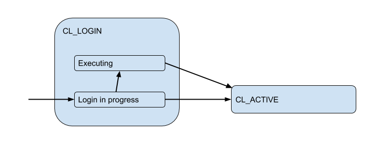

But these client connections are actually matched with backend / upstream database connections that PgBouncer opens within the pool and holds a limited amount. And they give the client such a connection only for a while - for the duration of the session, transaction or request, depending on the type of pooling (determined by the pool_mode setting). The most commonly used transaction pooling (we will mostly discuss this further) is when the connection is issued to the client for one transaction, and the rest of the time the client is not connected to the server after the fact. Thus, the client’s “active” state doesn’t tell us much, and we’ll break it down into the substates: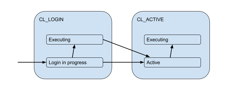

Each such client enters its own pool of connections, which will be issued for use by these connections to Postgres. This is the main task of PgBouncer to limit the number of connections to Postgres.

Due to the limited server connections, a situation may arise when the client needs to fulfill the request right now, but there is no free connection now. Then the client is queued and its connection enters the CL_WAITING state. Thus, the state diagram must be supplemented: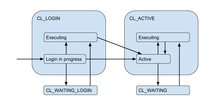

Since this can happen in the case when the client only logs in and needs to execute the request for authorization, the state CL_WAITING_LOGIN .

If you now look from the back side - from the server connections side, then they, respectively, are in such states: when authorization occurs immediately after the connection - SV_LOGIN , issued and (possibly) used by the client - SV_ACTIVE , or freely - SV_IDLE .

USE for PgBouncer

Thus, we come to the (naive version) Utilization of a specific pool:

 Pool utiliz =    /   

PgBouncer has a special pgbouncer service database in which there is a SHOW POOLS that shows the current states of the connections of each pool: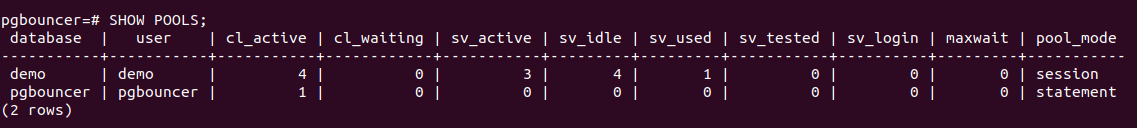

There are 4 client connections open and all are cl_active . Of the 5 server connections, there are 4 sv_active and one in the new state sv_used .

Naively removing metrics from SHOW POOLS (by some prometheus exporter) we can plot these states:

But to get to the disposal you need to answer a few questions:

• What is the size of the pool?
• How to count how many compounds are used? In jokes or in time, on average or in peak?

Pool size

It's all complicated, as in life. In total, there are already five limit settings in the pbbaunser!

• pool_size can be set for each base. A separate pool is created for each DB / user pair, i.e. from any additional user, you can create another pool_size pool_size backend / worker. Since if pool_size not set, it is folded in default_pool_size , which is by default 20, then it turns out that each user with connection rights to the database (and working through pgbouncer) can potentially create 20 Postgres processes, which is not much. But if you have many different user bases or the bases themselves, and the pools are not registered with a fixed user, i.e. will be created on the fly (and then deleted by autodb_idle_timeout ), then it can be dangerous =)
  

  Perhaps it is worth leaving the default_pool_size small, just for fire.
  

• max_db_connections - just needed to limit the total number of connections to one database, since otherwise, badly behaving, clients can create a lot of backends / postgres processes. And by default here - unlimited ¯_ (ツ) _ / ¯
  

  It may be worth changing the default max_db_connections , for example, you can focus on the max_connections your Postgres (by default 100). But if you have a lot of PgBouncer's ...
  

• reserve_pool_size - in fact, if pool_size all used, then PgBouncer can open several more connections to the base. I understand this is done to cope with a surge load. We will come back to this.
• max_user_connections - This, on the contrary, is the limit of connections from one user to all databases, i.e. true if you have several bases and they go under the same user.
• max_client_conn - how many client connections a PgBouncer will accept at all. The default, as is customary, has a very strange value - 100. That is, it is assumed that if suddenly more than 100 clients are breaking, they just need to send the reset and almost everything silently at the TCP level (well, in the logs, it must be admitted, there will be "no more connections allowed (max_client_conn)").
  

  Perhaps it is worth making max_client_conn >> SUM ( pool_size' ) , for example, 10 times more.
  

In addition to SHOW POOLS service pseudo-base pgbouncer also provides the SHOW DATABASES , which shows the limits actually applied to a specific pool:

Server connections

Once again - how to measure how many compounds are used?
In jokes on average / peak / in time?

In practice, it is quite problematic to monitor the use of pools with a bouncer by common tools, since pgbouncer itself provides only a momentary picture, and how often do not do a survey, there is still the possibility of a wrong picture due to sampling. Here is a real example when, depending on when the exporter was working out - at the beginning of a minute or at the end - the picture of both open and used compounds changes fundamentally:

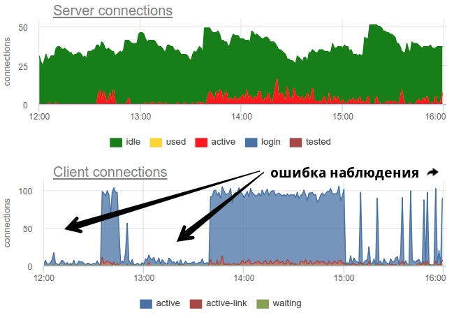
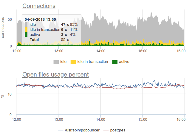
Here all the changes in the load / use of the connections are just a fiction, an artifact of the statistics collector restarts. Here you can look at the graphs of connections in Postgres for this time and on the file descriptors of the bouncer and PG - no changes:

Let's return to the issue of recycling. We in our service decided to use a combined approach - we sample SHOW POOLS once a second, and once a minute we render both the average and maximum number of connections in each state:

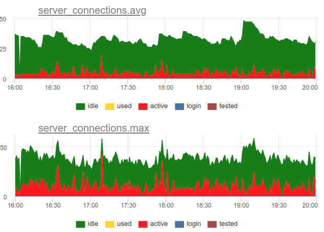
And if we divide the number of these active state connections by the size of the pool, we get the average and peak utilization of this pool and we can alert if it is close to 100%.

In addition, PgBouncer has a SHOW STATS command that will show usage statistics for each proxied database:

We are most interested in the total_query_time column - the time spent by all connections in the process of executing queries in postgres. And since version 1.8, there is also a total_xact_time metric - time spent in transactions. Based on these metrics, we can build the utilization of server connection time; this indicator is not subject, in contrast to the calculations calculated from the state of connections, to sampling problems, since these total_..._time counters are cumulative and do not miss anything:

Compare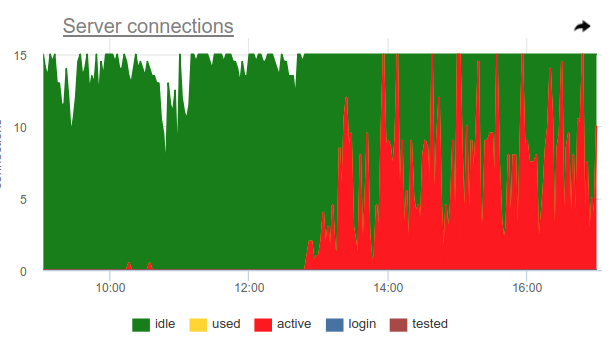

It can be seen that sampling does not show all moments of high ~ 100% utilization, and query_time shows.

Saturation and PgBouncer

Why do we need to keep track of Saturation, because by high utilization it is already clear that everything is bad?

The problem is that no matter how measured the recycling, even the accumulated counters cannot show the local 100% use of the resource if it occurs only at very short intervals. For example, you have any crowns or other synchronous processes that can simultaneously begin to make requests to the base on command. If these requests are short, then recycling, measured on the scale of a minute or even a second, may be low, but at the same time these requests were forced to wait for the queue to be executed. It seems that the situation is not 100% CPU usage and high Load average - it seems that CPU time is still there, but nevertheless many processes are waiting in the queue for execution.

How can you track such a situation - well, again, we can simply count the number of clients in the cl_waiting state according to SHOW POOLS . In a normal situation, such - zero, and more than zero means overflowing this pool:

There remains a problem with the fact that SHOW POOLS can only be sampled, and in a situation with synchronous crowns or something like that, we can simply skip and not see such waiting clients.

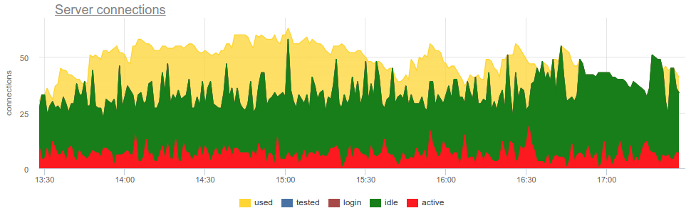
You can use this trick, pgbouncer can detect 100% use of the pool itself and open a backup pool. Two settings are responsible for this: reserve_pool_size — for its size, as I said, and reserve_pool_timeout — how many seconds a client must have been waiting before using the backup pool. Thus, if we see on the server connection graph that the number of connections open before Postgres is greater than pool_size, then the pool saturation was like this:

Obviously, something like kroons makes many requests once per hour and completely occupies the pool. And even though we don’t see the moment when active connections exceed the pool_size limit, the pgbouncer still had to open additional connections.

Also on this graph, the work of setting up server_idle_timeout is clearly visible - after how much cease to keep and close connections that are not used. By default, this is 10 minutes, which we see on the chart - after active peaks at exactly 5:00, 6:00, etc. (according to cron 0 * * * * ), connections hang idle + used another 10 minutes and close.

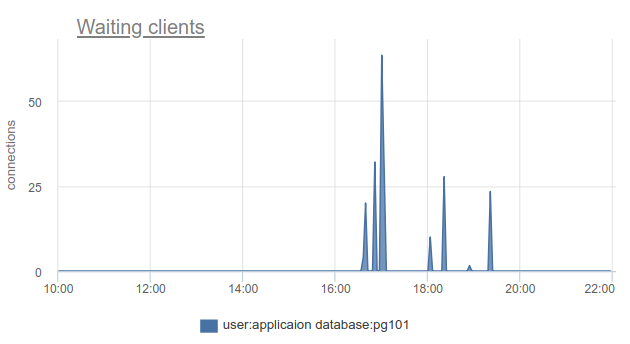
If you live on the cutting edge of progress and have updated PgBouncer over the past 9 months, you can find the total_wait_time column in SHOW STATS , which shows saturation best of all. cumulatively considers the time spent by customers in the waiting state. For example, here - the waiting appeared at 16:30: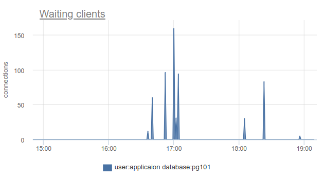

And wait_time , which is comparable and clearly affects the average query time , can be seen from 15:15 and almost to 19:

However, monitoring client connection states is still very useful, because allows you to find out not only the fact that all connections are spent on such a database and customers have to wait, but also because SHOW POOLS split into separate pools by users, and SHOW STATS does not, allows you to find out exactly which clients used all connections to a given base, by the sv_active column of the corresponding pool. Or by metric

 sum_by(user, database, metric(name="pgbouncer.clients.count", state="active-link")):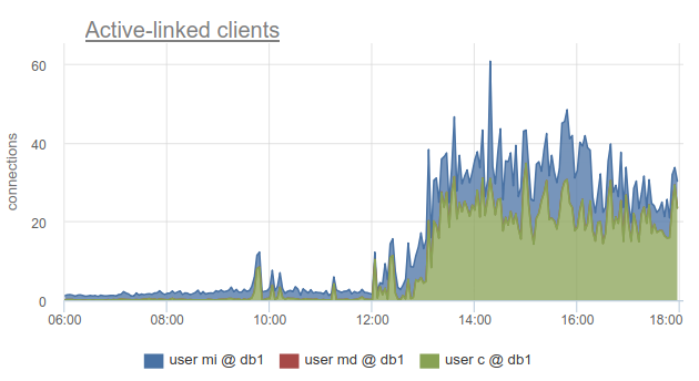 

We went even further into okmeter and added a breakdown of the connections used to the IP addresses of the clients who opened and used them. This allows you to understand which application instances behave differently:

Here we see aypishniki specific kubernetes pods with which you need to deal.

Errors

There is nothing particularly tricky here: pgbouncer writes logs in which it reports errors if the limit of client connections is reached, the timeout for connecting to the server, etc. So far we haven't gotten to the pgbouncer logs :(

RED for PgBouncer

While USE is more focused on performance, in the sense of bottlenecks, RED, in my opinion, is more about the characteristics of incoming and outgoing traffic in general, and not about bottlenecks. That is, RED answers the question - does everything work fine, and if not, then USE will help you to understand the problem.

Requests

It would seem that everything is quite simple for a SQL database and for a proxy / connection puller to such a database - clients execute SQL statements, which are Requests. From SHOW STATS we take total_requests and build a graph of its time derivative.

 rate(metric(name="pgbouncer.total_requests", database: "*")) 

But in fact there are different modes of pulling, and the most common is transactions. The unit of operation of this mode is a transaction, not a request. In accordance with this, starting from version 1.8, Pgbouner has already provided two other statistics - total_query_count , instead of total_requests , and total_xact_count - the number of past transactions.

Now workload can be characterized not only in terms of the number of completed requests / transactions, but you can, for example, look at the average number of requests per transaction into different databases, dividing one into another

 rate(metric(name="total_requests", database="*")) / rate(metric(name="total_xact", database="*")) 

Here we see obvious changes in the load profile, which may be the reason for the change in performance. And if they were looking only at the rate of transactions or requests, they could not see it.

RED Errors

It is clear that RED and USE overlap in error monitoring, but it seems to me that errors in USE are mostly about request processing errors due to 100% utilization, i.e. when the service refuses to take more work. And errors for RED would be better to measure errors from the point of view of the client, client requests. That is, not only in a situation when the pool in PgBouncer is full or another limit has been triggered, but also when request timeouts have been triggered, such as "canceling statement due to statement timeout", cancel'y and rollback and transactions by the client itself, t. e. higher-level, closer to the business logic types of errors.

Durations

SHOW STATS with cumulative total_xact_time , total_query_time and total_wait_time counters will help us again, dividing that by the number of requests and transactions, respectively, we get the average request time, average transaction time, average wait time per transaction. I already showed the schedule about the first and third:

What is there more to get? The well-known anti-pattern in working with the database and Postgres in particular, when an application opens a transaction, makes a request, then starts (long) to process its results or worse, goes to some other service / base and makes there requests. All this time, the transaction "hangs" in the open state, the service then returns and makes some more requests, updates in the database and only then closes the transaction. For postgres it is especially unpleasant, because pg workers are expensive. So, we can monitor when such an application resides idle in transaction in the post- state itself - in the state column in pg_stat_activity , but there all the same described problems with sampling, since pg_stat_activity gives only the current picture. In PgBouncer, we can subtract the time spent by customers in total_query_time requests from the time spent in transactions total_xact_time - this will be the time of such idling. If the result is still divided by total_xact_time , then it will be normalized: the value 1 corresponds to the situation when customers are idle in transaction 100% of the time. And with such a normalization, it makes it easy to understand how bad everything is:

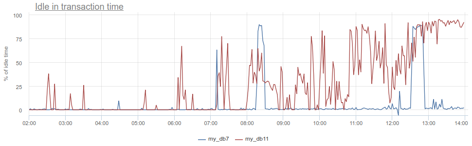
In addition, returning to Duration, the total_xact_time - total_query_time can be divided by the number of transactions to see how much the average idle application is per transaction.

In my opinion, USE / RED methods are most useful for structuring which metrics you are shooting and why. Since we are monitoring full-time and we have to do monitoring for various components of the infrastructure, these methods help us to remove the correct metrics, make the right schedules and triggers for our clients.

Good monitoring cannot be done right away, this is an iterative process. We in okmeter.io just continuous monitoring (a lot of things, but tomorrow will be better and more detailed :)