The blessed memory of my teacher - the first dean of the Faculty of Mathematics and Physics of the Novocherkassk Polytechnic Institute, Head of the Department "Theoretical Mechanics" Alexander N. Kabelkov

Introduction

August, summer is coming to an end. People violently rushed to the sea, but it is not surprising - the season. And on Habré, meanwhile, with pompous color it dissolves and smells of pseudoscience . If we talk about the topic of this issue of "Modeling ...", then we will combine the pleasant with the useful in it - we will continue the promised cycle and just a bit more will fight with this very pseudoscience for the inquisitive minds of modern youth.


And the question is really not idle - from school years we used to think that our closest satellite in outer space - the Moon moves around the Earth with a period of 29.5 days, especially without going into the accompanying details. In fact, our neighbor is a peculiar and to some extent unique astronomical object, with the movement of which around the Earth is not so simple as it might have been desirable for some of my colleagues from the near abroad.
')
So, leaving the controversy aside, we will try from different sides, to the best of our competence, to consider this unconditionally beautiful, interesting and very revealing task.

1. The law of world wideness and what conclusions we can make of it

Discovered in the second half of the 17th century, by Sir Isaac Newton, the law of universal perception speaks of the fact that the moon is attracted to the Earth (and the Earth to the Moon!) With a force directed along the straight line connecting the centers of the considered celestial bodies and equal to

$$

$$F_ {1,2} = G \, \ frac {m_1 \, m_2} {r_ {1,2} ^ 2}$$

where m ₁ , m ₂ are the masses, respectively, of the Moon and the Earth; G = 6.67e-11 m ³ / (kg * s ² ) - gravitational constant; r _1,2 is the distance between the centers of the moon and the earth. If we take into account only this force, then, having solved the problem of the motion of the Moon as a satellite of the Earth and having learned to calculate the position of the Moon in the sky against the background of stars, we will soon be convinced by direct measurements of the equatorial coordinates of the Moon that in our conservatory not everything is as smooth as I would like to. And the point here is not in the law of universal perception (and in the early stages of the development of celestial mechanics such thoughts were expressed quite often), but in unaccounted perturbation of the motion of the moon by other bodies. What kind? We look at the sky and our gaze immediately rests on a hefty, weighing as much as 1.99e30 kilograms plasma ball right under our nose - the Sun. Is the moon attracted to the sun? More like, with a force equal in magnitude

$$

$$F_ {1,3} = G \, \ frac {m_1 \, m_3} {r_ {1,3} ^ 2}$$

where m ₃ is the mass of the Sun; r _1,3 is the distance from the moon to the sun. Compare this force with the previous one.

$$

$$\ frac {F_ {1,3}} {F_ {1,2}} = \ frac {G \, \ frac {m_1 \, m_3} {r_ {1,3} ^ 2}} {G \, \ frac {m_1 \, m_2} {r_ {1,2} ^ 2}} = \ frac {m_3} {m_2} \, \ left (\ frac {r_ {1,2}} {r_ {1,3}} \ right) ^ 2$$

Take the position of the bodies, in which the attraction of the Moon to the Sun will be minimal: all three bodies are on one straight line and the Earth is located between the Moon and the Sun. In this case, our formula will look like:

$$

$$\ frac {F_ {1,3}} {F_ {1,2}} = \ frac {m_3} {m_2} \, \ left (\ frac {\ rho} {a + \ rho} \ right) ^ 2$$

Where $$$\ rho = 3,844 \ cdot 10 ^ {8}$ , m - the average distance from the Earth to the Moon; $$$a = 1,496 \ cdot10 ^ {11}$ , m - the average distance from the Earth to the Sun. Substitute the real parameters in this formula

$$

$$\ frac {F_ {1,3}} {F_ {1,2}} = \ frac {1.99 \ cdot 10 ^ {30} {5.98 \ cdot10 ^ {24}} \, \ left (\ frac {3.844 \ cdot10 ^ {8}} {1.496 \ cdot10 ^ {11} + 3.844 \ cdot10 ^ {8}} \ right) ^ 2 = 2.19$$

Here is the number! It turns out that the Moon is attracted to the Sun by a force that is more than two times greater than the force of its attraction to the Earth.

Such a disturbance can no longer be ignored, and it will definitely affect the final trajectory of the Moon. Let us go further, taking into account the assumption that the Earth’s orbit is circular with radius a, we find the locus of points around the Earth, where the force of attraction of any object to the Earth is equal to the force of its attraction to the Sun. This will be a sphere with a radius

$$

$$R = \ frac {a \, \ sqrt {\ gamma}} {1 - \ gamma}$$

displaced along a straight line connecting the Earth and the Sun in the opposite direction to the Sun at a distance

$$

$$l = R \, \ sqrt {\ gamma}$$

Where $$$\ gamma = m_2 / m_3$ - The ratio of the mass of the earth to the mass of the sun. Substituting the numerical values ​​of the parameters, we obtain the actual dimensions of this area: R = 259300 kilometers, and l = 450 kilometers. This sphere is called the sphere of the Earth relative to the Sun.

The known orbit of the moon lies outside this area. That is, at any point of the trajectory, the Moon suffers from the Sun significantly more attraction than from the Earth.

2. Satellite or planet? Gravitational scope

This information often gives rise to disputes that the Moon is not a satellite of the Earth, but an independent planet of the Solar System, whose orbit is outraged by the attraction of the near Earth.

Let us estimate the perturbation introduced by the Sun into the trajectory of the Moon relative to the Earth, as well as the disturbance introduced by the Earth into the trajectory of the Moon relative to the Sun, using the criterion proposed by P. Laplace. Consider three bodies: the Sun (S), the Earth (E) and the Moon (M).
Let us assume that the orbits of the Earth relative to the Sun and the Moon relative to the Earth are circular.


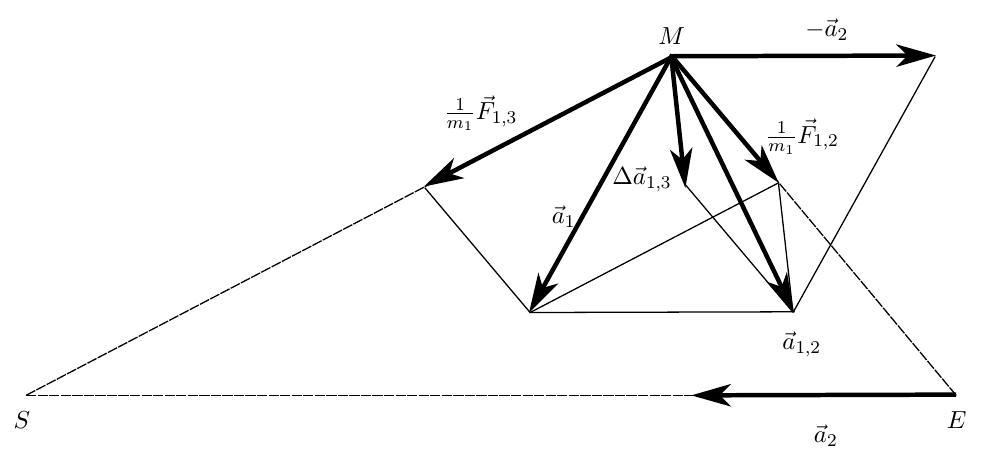
Consider the motion of the moon in a geocentric inertial frame of reference. The absolute acceleration of the moon in the heliocentric reference system is determined by the forces acting on it and is equal to:

$$

$$\ vec a_1 = \ vec a_1 ^ {(3)} + \ vec a_1 ^ {(2)} = \ frac {1} {m_1} \, \ vec F_ {1,3} + \ frac {1} { m_1} \, \ vec F_ {1,2}$$

On the other hand, according to the Coriolis theorem, the absolute acceleration of the moon

$$

$$\ vec a_1 = \ vec a_2 + \ vec a_ {1,2}$$

Where $$$\ vec a_2$ - portable acceleration equal to the acceleration of the Earth relative to the Sun; $$$\ vec a_ {1,2}$ - acceleration of the moon relative to the earth. Accelerations of Coriolis will not be here - the chosen coordinate system moves progressively. Hence we get the acceleration of the moon relative to the earth.

$$

$$\ vec a_ {1,2} = \ frac {1} {m_1} \, \ vec F_ {1,3} + \ frac {1} {m_1} \, \ vec F_ {1,2} - \ vec a_2$$

A portion of this acceleration equal to $$$\ vec a_1 ^ {(2)} = \ frac {1} {m_1} \, \ vec F_ {1,2}$ due to the attraction of the Moon to the Earth and characterizes its undisturbed geocentric movement. Remaining part

$$

$$\ Delta \ vec a_ {1,3} = \ frac {1} {m_1} \, \ vec F_ {1,3} - \ vec a_2$$

the acceleration of the moon caused by disturbance from the sun.

If we consider the motion of the moon in the heliocentric inertial reference frame, then everything is much simpler, the acceleration $$$\ vec a_1 ^ {(3)} = \ frac {1} {m_1} \, \ vec F_ {1,3}$ characterizes the undisturbed heliocentric motion of the moon, and the acceleration $$$\ Delta \ vec a_ {1,2} = \ frac {1} {m_1} \, \ vec F_ {1,2}$ - outrage of this movement from the Earth.

With the parameters of the orbits of the Earth and the Moon existing in the current epoch, the inequality is true at each point of the trajectory of the Moon

$$

$$\ frac {| \ Delta \ vec a_ {1,3} |} {| \ vec a_ {1} ^ {(2)} |} <\ frac {| \ Delta \ vec a_ {1,2} |} {| \ vec a_ {1} ^ {(3)} |} \ quad \ quad (1)$$

which can be verified by direct calculation, but I refer to the source in order not to overly clutter the article.

What does inequality (1) mean? Yes, the fact that in relative terms the effect of perturbation of the Moon by the Sun (and very significantly) is less than the effect of the attraction of the Moon to the Earth. And vice versa, the Earth's perturbation of the geoliocentric trajectory of the Moon has a decisive influence on the nature of its movement. The influence of the earth's gravity in this case is more significant, which means the moon "belongs" to the earth by right and is its satellite.

Another interesting thing is that by turning inequality (1) into an equation, you can find the locus of points where the effects of perturbations of the Moon (and any other body) by the Earth and the Sun are the same. Unfortunately, this is not so easy as in the case of the realm of the sphere. Calculations show that this surface is described by an equation of crazy order, but close to an ellipsoid of revolution. All that we can do without unnecessary problems is to assess the overall dimensions of this surface relative to the center of the Earth. Numerically solving the equation

$$

$$\ frac {| \ Delta \ vec a_ {1,3} |} {| \ vec a_ {1} ^ {(2)} |} = \ frac {| \ Delta \ vec a_ {1,2} |} {| \ vec a_ {1} ^ {(3)} |} \ quad \ quad (2)$$

relative to the distance from the center of the Earth to the desired surface on a sufficient number of points, we obtain the cross section of the desired surface by the ecliptic plane


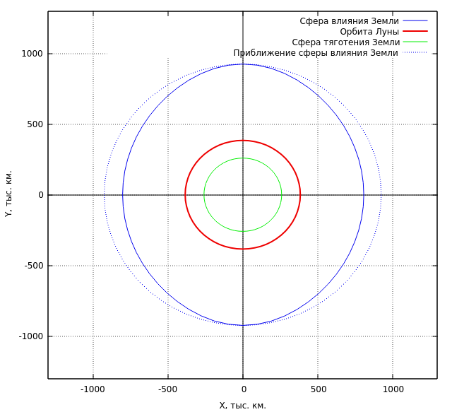
For clarity, the geocentric orbit of the moon is shown here, and the sphere we found above is relative to the sun. It can be seen from the figure that the sphere of influence, or the sphere of the gravitational action of the Earth relative to the Sun, is the surface of rotation about the X axis, flattened along the straight line connecting the Earth and the Sun (along the axis of eclipses). The moon's orbit is deep inside this imaginary surface.

For practical calculations, this surface is conveniently approximated by a sphere with a center in the center of the Earth and a radius equal to

$$

$$r = a \, \ left (\ frac {m} {M} \ right) ^ {\ frac {2} {5}} \ quad \ quad (3)$$

where m is the mass of a smaller celestial body; M is the mass of the larger body, in the field of which the smaller body moves; a - the distance between the centers of bodies. In our case

$$

$$r = a \, \ left (\ frac {m_2} {m_3} \ right) ^ {\ frac {2} {5}} = 1.496 \ cdot10 ^ {11} \, \ left (\ frac {5.98 \ cdot10 ^ {24}} {1.99 \ cdot10 ^ {30}} \ right) ^ {\ frac {2} {5}} = 925000, \, km$$

This unfinished million kilometers is the theoretical limit beyond which the power of the old woman of the Earth does not extend - its influence on the trajectories of astronomical objects is so small that it can be neglected. So, to launch the Moon in a circular orbit at a distance of 38.4 million kilometers from the Earth (as some linguists do) does not work, it is physically impossible.

This sphere, for comparison, is shown in the figure by a blue dashed line. At estimated calculations, it is considered that the body inside this sphere will experience only from the side of the Earth. If the body is outside this sphere, we believe that the body moves in the field of the sun. In practical cosmonautics, a method of conjugation of conic sections is known, which makes it possible to approximately calculate the trajectory of a spacecraft using the solution of the two-body problem. In this case, all the space that the apparatus overcomes is divided into similar spheres of influence.

For example, it is now clear that in order to have a theoretical opportunity to perform maneuvers for entering a circumlunar orbit, the spacecraft must fall within the sphere of the Moon’s action relative to the Earth. Its radius is easy to calculate by the formula (3) and it is equal to 66 thousand kilometers.

Thus, the moon can rightly be considered a satellite of the Earth. However, due to the significant influence of the gravitational field of the Sun, it does not move in the central gravitational field, which means its trajectory is not a conic section.

3. The three-body problem in the classical formulation

So, we will consider a model problem in a general formulation, known in celestial mechanics as a three-body problem. Consider three bodies of arbitrary mass, arranged arbitrarily in space and moving exclusively under the action of forces of mutual gravitational attraction


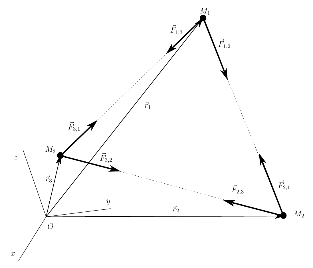
The bodies are considered material points. The position of the bodies will be counted in an arbitrary basis, which is associated with the inertial reference system Oxyz . The position of each of the bodies is given by the radius vector, respectively $$$\ vec r_1$ , $$$\ vec r_2$ and $$$\ vec r_3$ . Each body is affected by the force of gravitational attraction from the other two bodies, and in accordance with the third axiom of the dynamics of a point (Newton's 3rd law)

$$

$$\ vec F_ {i, j} = - \ vec F_ {j, i} \ quad \ quad (4)$$

We write the differential equations of motion of each point in vector form.

$$

$$\ begin {align} & m_1 \, \ frac {d ^ 2 \ vec r_1} {dt ^ 2} = \ vec F_ {1,2} + \ vec F_ {1,3} \\ & m_2 \, \ frac {d ^ 2 \ vec r_2} {dt ^ 2} = \ vec F_ {2,1} + \ vec F_ {2,3} \\ & m_3 \, \ frac {d ^ 2 \ vec r_3} {dt ^ 2} = \ vec F_ {3,1} + \ vec F_ {3,2} \ end {align}$$

or, taking into account (4)

$$

$$\ begin {align} & m_1 \, \ frac {d ^ 2 \ vec r_1} {dt ^ 2} = \ vec F_ {1,2} + \ vec F_ {1,3} \\ & m_2 \, \ frac {d ^ 2 \ vec r_2} {dt ^ 2} = - \ vec F_ {1,2} + \ vec F_ {2,3} \\ & m_3 \, \ frac {d ^ 2 \ vec r_3} { dt ^ 2} = - \ vec F_ {1,3} - \ vec F_ {2,3} \ end {align}$$

In accordance with the law of the world, the interaction forces are directed along the vectors

$$

$$\ begin {align} & \ vec r_ {1,2} = \ vec r_2 - \ vec r_1 \\ & \ vec r_ {1,3} = \ vec r_3 - \ vec r_1 \\ & \ vec r_ {2 , 3} = \ vec r_3 - \ vec r_2 \\ \ end {align}$$

Along each of these vectors we will release the corresponding ort

$$

$$\ vec e_ {i, j} = \ frac {1} {r_ {i, j}} \, \ vec r_ {i, j}$$

then each of the gravitational forces is calculated by the formula

$$

$$\ vec F_ {i, j} = G \, \ frac {m_i \, m_j} {r_ {i, j} ^ 2} \, \ vec e_ {i, j}$$

Given all this, the system of equations of motion takes the form

$$

$$\ begin {align} & \ frac {d ^ 2 \ vec r_1} {dt ^ 2} = \ frac {G \, m_2} {r_ {1,2} ^ 3} \, \ vec r_ {1,2 } + \ frac {G \, m_3} {r_ {1,3} ^ 3} \, \ vec r_ {1,3} \\ & \ frac {d ^ 2 \ vec r_2} {dt ^ 2} = - \ frac {G \, m_1} {r_ {1,2} ^ 3} \, \ vec r_ {1,2} + \ frac {G \, m_3} {r_ {2,3} ^ 3} \, \ vec r_ {2,3} \\ & \ frac {d ^ 2 \ vec r_3} {dt ^ 2} = - \ frac {G \, m_1} {r_ {1,3} ^ 3} \, \ vec r_ {1,3} - \ frac {G \, m_2} {r_ {2,3} ^ 3} \, \ vec r_ {2,3} \ end {align}$$

We introduce the notation adopted in celestial mechanics.

$$

$$\ mu_i = G \, m_i$$

- gravitational parameter of the attracting center. Then the equations of motion will take the final vector view.

$$

$$\ begin {align} & \ frac {d ^ 2 \ vec r_1} {dt ^ 2} = \ frac {\ mu_2} {r_ {1,2} ^ 3} \, \ vec r_ {1,2} + \ frac {\ mu_3} {r_ {1,3} ^ 3} \, \ vec r_ {1,3} \\ & \ frac {d ^ 2 \ vec r_2} {dt ^ 2} = - \ frac {\ mu_1} {r_ {1,2} ^ 3} \, \ vec r_ {1,2} + \ frac {\ mu_3} {r_ {2,3} ^ 3} \, \ vec r_ {2,3} \ \ & \ frac {d ^ 2 \ vec r_3} {dt ^ 2} = - \ frac {\ mu_1} {r_ {1,3} ^ 3} \, \ vec r_ {1,3} - \ frac {\ mu_2} {r_ {2,3} ^ 3} \, \ vec r_ {2,3} \ end {align}$$

4. Rationing of equations to dimensionless variables

A fairly popular technique in mathematical modeling is to reduce differential equations and other relations describing the process to dimensionless phase coordinates and dimensionless time. Other parameters are also normalized. This allows us to consider, albeit with the use of numerical modeling, but in a fairly general form a whole class of typical tasks. I leave the question of how justified this is in each solvable problem, but I agree that in this case, this approach is quite fair.

So, we introduce some abstract celestial body with a gravitational parameter $$$\ mu$ such that the orbital period of the satellite in an elliptical orbit with the major semiaxis $$$a$ around it is equal $$$T$ . All these quantities, by virtue of the laws of mechanics, are related by

$$

$$T = 2 \, \ pi \, \ left (\ frac {a ^ 3} {\ mu} \ right) ^ {\ frac {1} {2}}$$

We introduce the replacement of parameters. For the position of the points of our system

$$

$$\ vec r_i = a \, \ vec \ xi_i$$

Where $$$\ vec \ xi_i$ - dimensionless radius vector of the i-th point;
for gravity body parameters

$$

$$\ mu_i = \ varkappa_i \, \ mu$$

Where $$$\ varkappa_i$ - dimensionless gravitational parameter of the i-th point;
for time

$$

$$t = T \, \ tau$$

Where $$$\ tau$ - dimensionless time.

Now recalculate the acceleration points of the system through these dimensionless parameters. Let's apply direct double differentiation in time. For speeds

$$

$$\ vec v_i = \ frac {d \ vec r_i} {dt} = a \, \ frac {d \ vec \ xi_i} {dt} = \ frac {a} {T} \, \ frac {d \ vec \ xi_i} {d \ tau} = \ frac {1} {2 \, \ pi} \, \ sqrt {\ frac {\ mu} {a}} \, \ frac {d \ vec \ xi_i} {d \ tau }.$$

For acceleration

$$

$$\ vec a_i = \ frac {d \ vec v_i} {dt} = \ frac {1} {2 \, \ pi} \, \ sqrt {\ frac {\ mu} {a}} \, \ frac {1 } {dt} \ left (\ frac {d \ vec \ xi_i} {d \ tau} \ right) = \ frac {1} {4 \, \ pi ^ 2} \, \ frac {\ mu} {a ^ 2} \, \ frac {d ^ 2 \ vec \ xi_i} {d \ tau ^ 2}$$

When substituting the obtained relations into the equations of motion, everything elegantly collapses into beautiful equations:

$$

$$\ begin {align} & \ frac {d ^ 2 \ vec \ xi_1} {d \ tau ^ 2} = 4 \, \ pi ^ 2 \, \ varkappa_2 \, \ frac {\ vec \ xi_2 - \ vec \ xi_1} {| \ vec \ xi_2 - \ vec \ xi_1 | ^ 3} + 4 \, \ pi ^ 2 \, \ varkappa_3 \, \ frac {\ vec \ xi_3 - \ vec \ xi_1} {| \ vec \ xi_3 - \ vec \ xi_1 | ^ 3} \\ & \ frac {d ^ 2 \ vec \ xi_2} {d \ tau ^ 2} = -4 \, \ pi ^ 2 \, \ varkappa_1 \, \ frac {\ vec \ xi_2 - \ vec \ xi_1} {| \ vec \ xi_2 - \ vec \ xi_1 | ^ 3} + 4 \, \ pi ^ 2 \, \ varkappa_3 \, \ frac {\ vec \ xi_3 - \ vec \ xi_2} {| \ vec \ xi_3 - \ vec \ xi_2 | ^ 3} \ quad \ quad (5) \\ & \ frac {d ^ 2 \ vec \ xi_3} {d \ tau ^ 2} = -4 \, \ pi ^ 2 \, \ varkappa_1 \, \ frac {\ vec \ xi_3 - \ vec \ xi_1} {| \ vec \ xi_3 - \ vec \ xi_1 | ^ 3} - 4 \, \ pi ^ 2 \, \ varkappa_2 \, \ frac {\ vec \ xi_3 - \ vec \ xi_2} {| \ vec \ xi_3 - \ vec \ xi_2 | ^ 3} \ end {align}$$

This system of equations is still considered non-integrable in analytic functions. Why is it considered and is not? Because the successes of the theory of the function of a complex variable led to the fact that the general solution of the three-body problem did appear in 1912 — Karl Sundman found an algorithm for finding coefficients for infinite series with respect to a complex parameter, which theoretically is a general solution of the three-body problem. But ... for the application of Zundman's series in practical calculations with the accuracy required for them, it requires obtaining such a number of members of these series that this task is much greater than the capabilities of computers even today.

Therefore, numerical integration is the only way to analyze the solution of equation (5)

5. Calculation of the initial conditions: extract the source data

As I wrote earlier , before starting the numerical integration, you should take care to calculate the initial conditions for the problem to be solved. In the problem under consideration, the search for initial conditions turns into an independent subtask, since system (5) gives us nine second-order scalar equations, which, when going to normal form, Cauchy increases the order of the system by another 2 times. That is, we need to calculate as many as 18 parameters — the initial positions and components of the initial velocity of all points of the system. Where do we get data on the position of the celestial bodies of interest to us? We live in a world where man walked on the moon - naturally, humanity must have information about how this moon moves and where it is located.

That is, you say, you, dude, offer us to take thick astronomical reference books from the shelves, blow dust from them ... They didn’t guess! I propose to go for these data to those who actually walked on the moon, to NASA, namely in the Jet Propulsion Laboratory, Pasadena, California. Here is the JPL Horizonts web interface .

Here, having spent some time studying the interface, we will get all the data we need. Choose a date, for example, yes we do not care, but let it be July 27, 2018 UT 20:21. Just at that moment there was a complete phase of the lunar eclipse. The program will give us a huge footwoman


Br-rr, what is it? Without panic, for someone who taught astronomy well at school, there is nothing to fear for mechanics and mathematics. So, the most important final search coordinates and components of the velocity of the moon.

 $$SOE 2458327.347916670 = AD 2018-Jul-27 20:21:00.0003 TDB X = 1.537109094089627E-03 Y =-2.237488447258137E-03 Z = 5.112037386426180E-06 VX= 4.593816208618667E-04 VY= 3.187527302531735E-04 VZ=-5.183707711777675E-05 LT= 1.567825598846416E-05 RG= 2.714605874095336E-03 RR=-2.707898607099066E-06 $$EOE 

Yes, yes, yes, they are Cartesian! If you carefully read the entire footcloth, then we learn that the origin of this coordinate system coincides with the center of the Earth. The XY plane lies in the plane of the earth's orbit (the plane of the ecliptic) for the epoch J2000. The X axis is directed along the line of intersection of the equatorial plane of the Earth and the ecliptic to the vernal equinox.The Z axis looks in the direction of the north pole of the Earth perpendicular to the plane of the ecliptic. Well, the Y axis complements all this happiness to the right three vectors. By default, the units of measurement of coordinates are astronomical units (the clever ones from NASA also give the value of the autronomic unit in kilometers). Speed ​​units: astronomical units per day, day is assumed to be 86400 seconds. Full stuffing!

Similar information can be obtained for the Earth.


Here, the barycenter (center of mass) of the Solar system is chosen as the origin of coordinates. The data we are interested in

 $$SOE 2458327.347916670 = AD 2018-Jul-27 20:21:00.0003 TDB X = 5.755663665315949E-01 Y =-8.298818915224488E-01 Z =-5.366994499016168E-05 VX= 1.388633512282171E-02 VY= 9.678934168415631E-03 VZ= 3.429889230737491E-07 LT= 5.832932117417083E-03 RG= 1.009940888883960E+00 RR=-3.947237246302148E-05 $$EOE 

For the moon, we will need the coordinates and speed relative to the barycenter of the solar system, we can calculate them, or we can ask NASA to give us such data

 $$SOE 2458327.347916670 = AD 2018-Jul-27 20:21:00.0003 TDB X = 5.771034756256845E-01 Y =-8.321193799697072E-01 Z =-4.855790760378579E-05 VX= 1.434571674368357E-02 VY= 9.997686898668805E-03 VZ=-5.149408819470315E-05 LT= 5.848610189172283E-03 RG= 1.012655462859054E+00 RR=-3.979984423450087E-05 $$EOE 

Wonderful! Now it is necessary to slightly process the received data with a file.

6. 38 parrots and one parrot wing

To begin with, we will define the scale, because our equations of motion (5) are written in dimensionless form. The data provided by NASA themselves tell us that for the scale of the coordinates is to take one astronomical unit. Accordingly, as a reference body, to which we will ration the masses of other bodies, we take the Sun, and as the time scale, the period of the Earth’s orbit around the Sun.

All this is of course very good, but we did not set the initial conditions for the sun. “Why?” Some linguist would ask me. And I would say that the Sun is not motionless at all, but also rotates in its orbit around the center of mass of the Solar system. This can be seen by looking at the NASA data for the sun.

 $$SOE 2458327.347916670 = AD 2018-Jul-27 20:21:00.0003 TDB X = 6.520050993518213E+04 Y = 1.049687363172734E+06 Z =-1.304404963058507E+04 VX=-1.265326939350981E-02 VY= 5.853475278436883E-03 VZ= 3.136673455633667E-04 LT= 3.508397935601254E+00 RG= 1.051791240756026E+06 RR= 5.053500842402456E-03 $$EOE 

Looking at the RG parameter, we will see that the Sun rotates around the solar system barycenter, and as of 07/27/2018, the center of the star is at a distance of one million kilometers. The radius of the sun, for reference - 696 thousand kilometers. That is, the barycenter of the solar system lies half a million kilometers from the surface of the star. Why?Yes, because all other bodies interacting with the Sun also inform him of the acceleration, mainly, of course, the heavy Jupiter. Accordingly, the Sun also has its own orbit.

Of course, we can choose these data as initial conditions, but no - we solve the three-body model problem, and Jupiter and other characters are not included in it. So to the detriment of realism, knowing the position and velocity of the Earth and the Moon, we recalculate the initial conditions for the Sun, so that the center of mass of the Sun-Earth-Moon system is at the origin. For the center of mass of our mechanical system, the equation

$$

$$(m_1 + m_2 + m_3) \, \vec r_C = m_1 \, \vec r_1 + m_2 \, \vec r_2 + m_3 \, \vec r_3$$

We place the center of mass at the origin, that is, let us set $$$\vec r_C = 0$ then

$$

$$m_1 \, \vec r_1 + m_2 \, \vec r_2 + m_3 \, \vec r_3 = 0$$

from where

$$

$$\begin{align} & m_3 \, \vec r_3 = -m_1 \, \vec r_1 - m_2 \, \vec r_2 \\ & \vec r_3 = - \frac{m_1}{m_3} \vec r_1 - \frac{m_2}{m_3} \, \vec r_2 \end{align}$$

We turn to the dimensionless coordinates and parameters by selecting $$$\mu = \mu_3$

$$

$$\vec \xi_3 = -\varkappa_1 \vec \xi_1 -\varkappa_2 \vec \xi_2\quad\quad(6)$$

Differentiating (6) over time and moving to dimensionless time, we also obtain the ratio for the velocities

$$

$$\vec u_3 = -\varkappa_1 \, \vec u_1 -\varkappa_2 \, \vec u_2$$

Where $$$\vec u_i = \cfrac{d\vec \xi_i}{d\tau}, \forall i=\overline{1,3}$

Now we will write a program that will form the initial conditions in the “parrots” we have chosen. What will we write on? Of course on Python! After all, as you know, this is the best language for mathematical modeling.

However, if we get away from sarcasm, then we will really try a python for this purpose, and why not? I will definitely provide a link to all the code in my Github profile .


Program exhaust

    mu[0] = 4901783000000.0 mu[1] = 386326400000000.0 mu[2] = 1.326663e+20    xi[0] = 3.6948215183509304e-08 xi[1] = 2.912016088486677e-06 xi[2] = 1.0   T = 31563683.35432583   , ..: [ 5.77103476e-01 -8.32119380e-01 -4.85579076e-05]   , ..: [ 5.75566367e-01 -8.29881892e-01 -5.36699450e-05]   , ..: [-1.69738146e-06 2.44737475e-06 1.58081871e-10]   , /: [24838.98933473 17310.56333294 -89.15979106] -//- : [ 5.24078311 3.65235907 -0.01881184]   , /: [2.40435899e+04 1.67586567e+04 5.93870516e-01] -//- : [5.07296163e+00 3.53591219e+00 1.25300854e-04]   , /: [-7.09330769e-02 -4.94410725e-02 1.56493465e-06] -//- : [-1.49661835e-05 -1.04315813e-05 3.30185861e-10] 

7. Integrating the equations of motion and analyzing the results

Actually, the integration itself boils down to a more or less standard for SciPy procedure for preparing a system of equations: transforming an ODE system to the Cauchy form and calling the corresponding solver functions. To transform the system into a Cauchy form, we recall that

$$

$$\vec u_i = \frac{d\vec \xi_i}{d\tau}, \forall i=\overline{1,3}\quad\quad(7)$$

Then by entering the system state vector

$$

$$\vec y = \left[\vec\xi_1, \vec\xi_2, \vec\xi_1, \vec u_1, \vec u_2, \vec u_3 \right]^T$$

we reduce (7) and (5) to one vector equation

$$

$$\frac{d\vec y}{d\tau} = \vec f(\tau, \vec y)\quad\quad(8)$$

To integrate (8) with the initial conditions, we write a little, quite a bit of code


Let's see what we did. The result was a spatial trajectory of the moon for the first 29 days from the chosen starting point.


as well as its projection into the ecliptic plane.


“Hey, uncle, what are you giving us?” It's a circle! ”

First, it’s not a circle - there is a noticeable shift in the projection of the trajectory from the origin to the right and down. Secondly - you notice nothing? No, well, really?


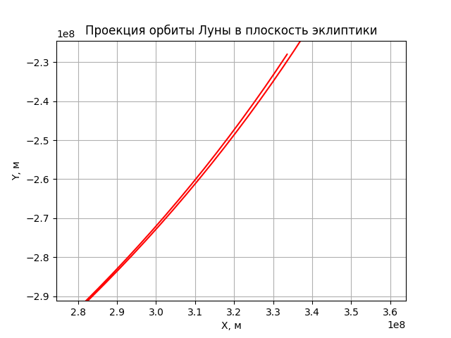
I promise to prepare a rationale for that (based on the analysis of the errors of the account and NASA data) that the resulting shift in the trajectory is not due to integration errors. While I suggest the reader to take my word for it - this shift is a consequence of the solar perturbation of the lunar trajectory. Spin one more turn



In both! And pay attention to the fact that, based on the initial data of the task, the Sun is just in that direction, where the trajectory of the Moon is shifted on each turn. Yes, this insolent Sun steals our favorite companion! Oh, this is the sun!

It can be concluded that solar gravity affects the moon's orbit quite significantly - the old woman does not walk twice through the sky in the same way. The picture for six months of movement allows (at least qualitatively) to make sure of this (the picture is clickable)



Interesting?Still would. Astronomy is generally entertaining science.

P.S

In the university where I studied and worked for almost seven years - the Novocherkassk Polytechnic Institute - an annual student Olympiad on the theoretical mechanics of universities in the North Caucasus was held annually. Three times we took the All-Russian Olympiad. At the opening, our main "Olympian", Professor Kondratenko AI, always said: "Academician Krylov called mechanics the poetry of the exact sciences."

I love mechanics. All the good things that I have achieved in my life and career have happened thanks to this science and my wonderful teachers. I respect the mechanics.

Therefore, I will never allow anyone to scoff at this science and brazenly exploit it for their own purposes to anyone, even if it is at least three times a PhD and a linguist four times, and has developed at least a million training programs. I sincerely believe that writing articles on a popular public resource should provide for their careful reading, normal design (LaTeX formulas are not the whim of resource developers!) And the absence of errors leading to results that violate the laws of nature. The latter is generally a “must have”.

I often tell my students: “The computer frees your hands, but this does not mean that you need to turn off the brain as well.”

I also urge you, my dear readers, to appreciate and respect the mechanics. I will gladly answer any questions, and the source code of the example of solving the three-body problem in Python, as promised,I post it on my Github profile .

Thanks for attention!