As we in 1C: Enterprise, we solve systems of algebraic equations
Working with numerical matrices in general and solving systems of linear algebraic equations in particular is a classical mathematical and algorithmic problem widely used in modeling and calculating a huge class of business processes (for example, when calculating the cost). When creating and operating 1C: Enterprise configurations, many developers faced the need to manually implement SLAE calculation algorithms, and then - the problem of long waiting for a solution.
"1C: Enterprise" 8.3.14 will contain functionality that allows you to significantly reduce the time to solve systems of linear equations by using an algorithm based on graph theory.
It is optimized for use on data having a sparse structure (that is, containing no more than 10% of nonzero coefficients in equations) and, on average and at best, demonstrates the asymptotics of Θ (n⋅log (n) log (n)), where n - the number of variables, and at worst (when the system is ~ 100% full), its asymptotics is comparable with classical algorithms (Θ (n 3 )). At the same time, on systems with ~ 10 5 unknowns, the algorithm shows acceleration hundreds of times as compared with those implemented in specialized libraries of linear algebra (for example, superlu or lapack ).
')

Important: the article and the described algorithm require an understanding of linear algebra and graph theory at the first-year level of the university.
Consider the simplest sparse system of linear equations:
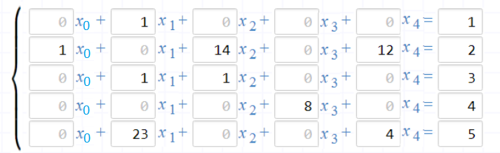
Attention: the system is randomly generated and will be used further to demonstrate the steps of the algorithm
At the first glance, an association with another mathematical object arises: the adjacency matrix of the graph. So why not convert data to adjacency lists, saving memory in the process of execution and speeding up access to non-zero coefficients?
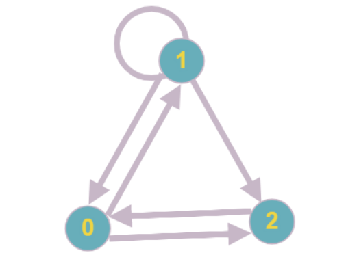
To do this, we just need to transpose the matrix and set the invariant “A [i] [j] = z-the i-th variable enters the j-th equation with the coefficient z” , and after each non-zero A [i] [j] build the corresponding edge from vertex i to vertex j.
The resulting graph will look like this:
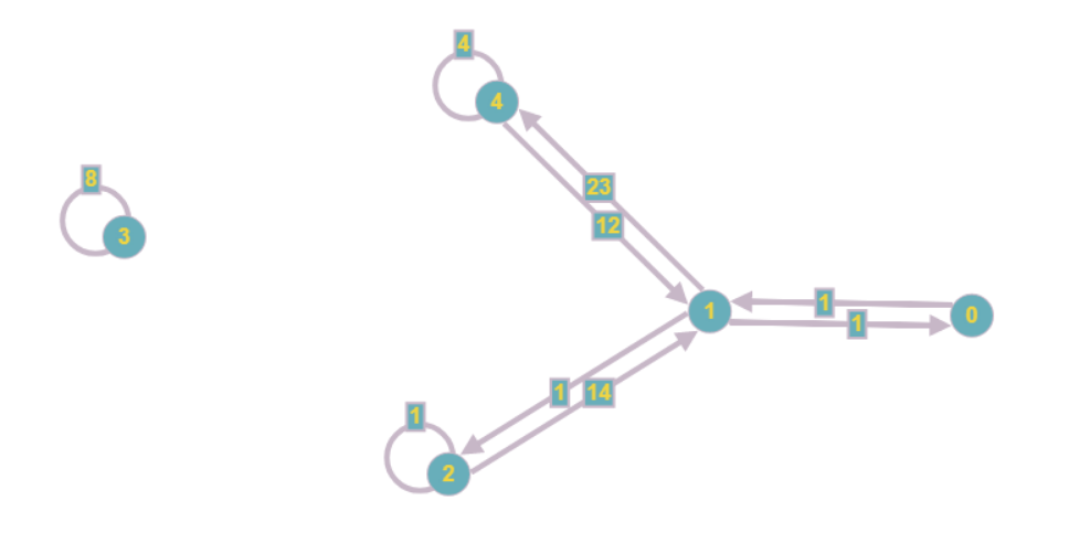
Even visually, it is less cumbersome, and the asymptotic cost of RAM is reduced from O (n 2 ) to O (n + m), where m is the number of coefficients in the system.
The second algorithmic idea that comes to mind when considering the resulting entity: the use of the principle of "divide and conquer." In terms of the graph, this leads to the separation of the set of vertices into weak connected components.
Let me remind you that a weakly connected component is such a subset of vertices, maximum by inclusion, that between any two there is a path from the edges in the undirected graph. We can get an undirected graph from the source graph, for example, by adding the opposite to each edge (followed by deletion). Then in one component of connectivity all vertices will be included, which we can reach by traversing the graph in depth.
After separation into weakly connected components, the graph takes the following form:
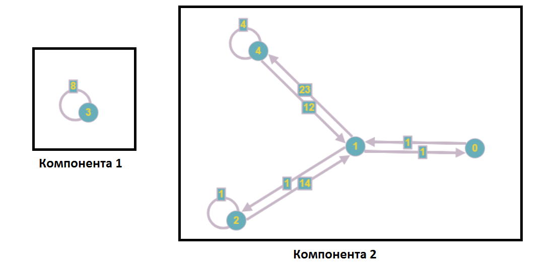
In the analysis of a system of linear equations, this means that not a single vertex from the first component enters the equations with the numbers of the second component and vice versa, that is, we can solve these subsystems independently (for example, in parallel).
The next step of the algorithm is exactly what the optimization for working with sparse matrices is. Even in the example graph, there are “hanging” vertices, meaning that some of the equations contain only one unknown and, as we know, the value of this unknown is easy to find.
To determine such equations, it is proposed to store an array of lists containing the numbers of variables included in the equation having the number of this element of the array. Then, when the list reaches a single size, we can reduce the very “single” vertex, and report the resulting value to the other equations in which this vertex enters.
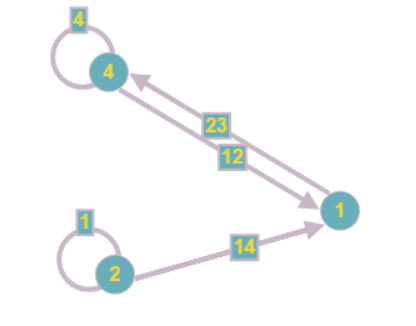
Thus, we will be able to reduce vertex 3 from the example immediately, having completely processed the component:
We will do the same with equation 0, since it includes only one variable:
Other equations also change after finding this result:
The graph takes the following form:
Note that when reducing one vertex, others may appear, also containing one unknown. So this step of the algorithm should be repeated as long as it is possible to reduce at least one of the vertices.
The most attentive readers may have noticed that a situation is possible in which each of the vertices of the graph will have a degree of occurrence of at least two and continue to gradually reduce the vertices will be impossible.
The simplest example of such a graph: each vertex has a degree of occurrence equal to two, none of the vertices can be reduced.
In the framework of optimization for sparse matrices, it is assumed that such subgraphs will be small in size, however, you will still have to work with them. To calculate the values of the unknowns included in the subsystem of equations, it is proposed to use classical methods for solving SLAEs (this is why the introduction states that with a matrix that has all or almost all the coefficients in the equations non-zero, our algorithm will have the same asymptotic complexity as the standard ).
For example, one can bring the set of vertices remaining after reduction back into the matrix view and apply the Gauss solution method to it. Thus, we get the exact solution, and the speed of the algorithm will be reduced by processing not the entire system, but only some of its parts.
To test the software implementation of the algorithm, we took several real systems of large-scale equations, as well as a large number of randomly generated systems.
The generation of a random system of equations passed through the successive addition of edges of arbitrary weight between two random vertices. Total system was filled by 5-10%. Verification of the correctness of the solutions was carried out by substituting the received answers into the original system of equations.

Systems ranged from 1000 to 200,000 unknowns.
To compare performance, we used the most popular libraries for solving linear algebra problems, such as superlu and lapack. Of course, these libraries are focused on solving a wide class of problems and the solution of the SLAE in them is not optimized in any way; therefore, the difference in speed was significant.
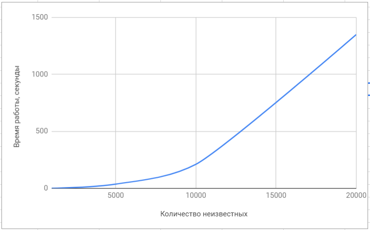
Testing the 'lapack' library
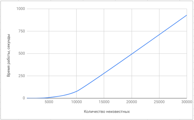
Testing the 'superlu' library
Here is a final comparison of our algorithm with algorithms implemented in popular libraries:

Even if you are not a developer of 1C: Enterprise configurations, the ideas and optimization methods described in this article can be used by you not only when implementing the SLAE solution algorithm, but also for a whole class of linear algebra problems related to matrices.
For 1C developers, we add that the new functionality of the SLAE solution supports parallel use of computational resources, and the number of computation threads used can be adjusted.
"1C: Enterprise" 8.3.14 will contain functionality that allows you to significantly reduce the time to solve systems of linear equations by using an algorithm based on graph theory.
It is optimized for use on data having a sparse structure (that is, containing no more than 10% of nonzero coefficients in equations) and, on average and at best, demonstrates the asymptotics of Θ (n⋅log (n) log (n)), where n - the number of variables, and at worst (when the system is ~ 100% full), its asymptotics is comparable with classical algorithms (Θ (n 3 )). At the same time, on systems with ~ 10 5 unknowns, the algorithm shows acceleration hundreds of times as compared with those implemented in specialized libraries of linear algebra (for example, superlu or lapack ).
')
Important: the article and the described algorithm require an understanding of linear algebra and graph theory at the first-year level of the university.
Representation of SLAE in the form of a graph
Consider the simplest sparse system of linear equations:
Attention: the system is randomly generated and will be used further to demonstrate the steps of the algorithm
At the first glance, an association with another mathematical object arises: the adjacency matrix of the graph. So why not convert data to adjacency lists, saving memory in the process of execution and speeding up access to non-zero coefficients?
To do this, we just need to transpose the matrix and set the invariant “A [i] [j] = z-the i-th variable enters the j-th equation with the coefficient z” , and after each non-zero A [i] [j] build the corresponding edge from vertex i to vertex j.
The resulting graph will look like this:
Even visually, it is less cumbersome, and the asymptotic cost of RAM is reduced from O (n 2 ) to O (n + m), where m is the number of coefficients in the system.
Selection of weakly connected components
The second algorithmic idea that comes to mind when considering the resulting entity: the use of the principle of "divide and conquer." In terms of the graph, this leads to the separation of the set of vertices into weak connected components.
Let me remind you that a weakly connected component is such a subset of vertices, maximum by inclusion, that between any two there is a path from the edges in the undirected graph. We can get an undirected graph from the source graph, for example, by adding the opposite to each edge (followed by deletion). Then in one component of connectivity all vertices will be included, which we can reach by traversing the graph in depth.
After separation into weakly connected components, the graph takes the following form:
In the analysis of a system of linear equations, this means that not a single vertex from the first component enters the equations with the numbers of the second component and vice versa, that is, we can solve these subsystems independently (for example, in parallel).
Reducing graph vertices
The next step of the algorithm is exactly what the optimization for working with sparse matrices is. Even in the example graph, there are “hanging” vertices, meaning that some of the equations contain only one unknown and, as we know, the value of this unknown is easy to find.
To determine such equations, it is proposed to store an array of lists containing the numbers of variables included in the equation having the number of this element of the array. Then, when the list reaches a single size, we can reduce the very “single” vertex, and report the resulting value to the other equations in which this vertex enters.
Thus, we will be able to reduce vertex 3 from the example immediately, having completely processed the component:
We will do the same with equation 0, since it includes only one variable:
Other equations also change after finding this result:
$$ display $$ 1⋅_1 + 1⋅_2 = 3⇒1⋅_2 = 3-1 = 2 $$ display $$
The graph takes the following form:
Note that when reducing one vertex, others may appear, also containing one unknown. So this step of the algorithm should be repeated as long as it is possible to reduce at least one of the vertices.
Rebuilding the graph
The most attentive readers may have noticed that a situation is possible in which each of the vertices of the graph will have a degree of occurrence of at least two and continue to gradually reduce the vertices will be impossible.
The simplest example of such a graph: each vertex has a degree of occurrence equal to two, none of the vertices can be reduced.
In the framework of optimization for sparse matrices, it is assumed that such subgraphs will be small in size, however, you will still have to work with them. To calculate the values of the unknowns included in the subsystem of equations, it is proposed to use classical methods for solving SLAEs (this is why the introduction states that with a matrix that has all or almost all the coefficients in the equations non-zero, our algorithm will have the same asymptotic complexity as the standard ).
For example, one can bring the set of vertices remaining after reduction back into the matrix view and apply the Gauss solution method to it. Thus, we get the exact solution, and the speed of the algorithm will be reduced by processing not the entire system, but only some of its parts.
Algorithm Testing
To test the software implementation of the algorithm, we took several real systems of large-scale equations, as well as a large number of randomly generated systems.
The generation of a random system of equations passed through the successive addition of edges of arbitrary weight between two random vertices. Total system was filled by 5-10%. Verification of the correctness of the solutions was carried out by substituting the received answers into the original system of equations.
Systems ranged from 1000 to 200,000 unknowns.
To compare performance, we used the most popular libraries for solving linear algebra problems, such as superlu and lapack. Of course, these libraries are focused on solving a wide class of problems and the solution of the SLAE in them is not optimized in any way; therefore, the difference in speed was significant.
Testing the 'lapack' library
Testing the 'superlu' library
Here is a final comparison of our algorithm with algorithms implemented in popular libraries:
Conclusion
Even if you are not a developer of 1C: Enterprise configurations, the ideas and optimization methods described in this article can be used by you not only when implementing the SLAE solution algorithm, but also for a whole class of linear algebra problems related to matrices.
For 1C developers, we add that the new functionality of the SLAE solution supports parallel use of computational resources, and the number of computation threads used can be adjusted.
Source: https://habr.com/ru/post/420029/
All Articles