How Python Helps Replace Financial Advisors
In continuation of the article on the dangers of excessive diversification, we will create useful tools for selecting stocks. After that, we will do a simple rebalancing and add unique conditions of technical indicators, which are so often lacking in popular services. And then we compare the profitability of individual assets and different portfolios.
In all this, we use Pandas and minimize the number of cycles. We group the time series and draw graphs. Let's get acquainted with multi-index and their behavior. And all this in Jupyter in Python 3.6.
The described tool will allow selecting the optimal assets for the portfolio and excluding instruments imposed by consultants. But we will see only a general picture - without taking into account liquidity, time for recruiting positions, broker commissions and the cost of one share. In general, with monthly or annual rebalancing of large brokers, this will be a minor cost. However, before applying the chosen strategy, it is still worth checking in the event-driven back tester, for example, Quantopian (QP), in order to eliminate potential errors.
Why not immediately in QP? Time. There the easiest test lasts about 5 minutes. And the current solution will allow you to check hundreds of different strategies with unique conditions in a minute.
')
To download the data, take the method described in this article . I use PostgreSQL to store daily prices, but now there are a lot of free sources from which you can generate the necessary DataFrame.
The code for downloading the price history from the database is available in the repository. The link will be at the end of the article.
When working with price history, for convenient grouping and access to all data, the best solution is to use the multi-index (MultiIndex) with the date and tickers.
Using a multi-index, we can easily access the entire price history for all assets and can group an array separately by date and asset. We can also get a price history for one asset.
Here is an example of how you can easily group history by week, month, and year. And all this is shown on the graphs by Pandas:
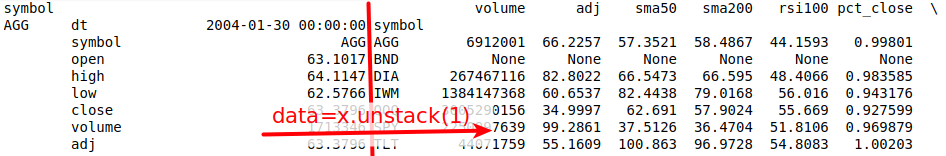
To correctly display the area with the chart legend, we move the index level with tickers to the second level above the columns using the Series (). Unstack (1) command. With DataFrame () this number will not work, but there is a solution below.
When grouping by standard periods, Pandas uses the latest calendar date of the group in the index, which is often different from actual dates. To fix this, update the index.
An example of getting the price history of a certain asset (we take all the dates, the ticker QQQ and all the columns):
Now we can see in a few lines on the chart the change in the price of each asset for the period of interest to us. To do this, we get the percentage change in price, grouping the dataframe by the multi-index level with the asset ticker.
Now we use the Series (). Rolling () window method and derive the return on assets for a certain period:
So we got to the most delicious. In the examples, we will look at the results of the portfolio in the allocation of capital on pre-determined shares between several assets. And also we will add unique conditions according to which we will refuse some assets at the moment of capital distribution. If there are no suitable assets, we will assume that the capital lies with the broker in the cache.
In order to use the Pandas methods when rebalancing, we need to store the distribution shares and the rebalancing conditions in the DataFrame with grouped data. Now consider the rebalancing functions that will be passed to the DataFrame (). Apply () method:
In order:
In the rebalancing functions, we need an array of all the data on the date in terms of assets. The DataFrame (). Apply () method, by which we will calculate the results of the portfolios, will pass an array to our function, where the columns will become an index of rows. And if we make a multi-index, where tickers are zero, then a multi-index will come to us. We will be able to expand this multi-index into a two-dimensional array and get the data of the corresponding asset on each line.
Now it’s enough to prepare the necessary conditions and make a calculation for each portfolio in a cycle. First of all, let's calculate the indicators on the daily price history:
Now group the history under the desired rebalancing period using the methods described above. We will take in this case the values of the indicators at the beginning of the period, in order to exclude peeping into the future.
We describe the structure of portfolios and indicate the necessary rebalancing. Portfolios are calculated in a cycle, since we need to specify unique shares and conditions:
This time we will need to turn the trick with the indexes of columns and rows to get the desired multi-index in the rebalancing function. We achieve this by calling the DataFrame (). Stack (). Unstack ([1, 2]) methods in succession. This code will transfer the columns to the lower-order multi-index, and then return the multi-index back with tickers and columns in the desired order.
Now it remains to draw everything. To do this, once again run a cycle of portfolios, which will display data on the graphs. In the end we draw SPY as a benchmark for comparison.
The considered code allows you to select different portfolio structures and rebalancing conditions. With it, you can quickly check whether, for example, it is worth holding gold (GLD) or emerging markets (EEM) in a portfolio. Try it yourself, add your own indicator conditions or select the parameters already described. (But remember the survivor’s mistake and that fitting to past data may not meet future expectations.) And after that, decide who you trust your portfolio to - Python or finco-sultant?
Repository: rebalance.portfolio
In all this, we use Pandas and minimize the number of cycles. We group the time series and draw graphs. Let's get acquainted with multi-index and their behavior. And all this in Jupyter in Python 3.6.
If you want to do something good, do it yourself.
Ferdinand Porsche
The described tool will allow selecting the optimal assets for the portfolio and excluding instruments imposed by consultants. But we will see only a general picture - without taking into account liquidity, time for recruiting positions, broker commissions and the cost of one share. In general, with monthly or annual rebalancing of large brokers, this will be a minor cost. However, before applying the chosen strategy, it is still worth checking in the event-driven back tester, for example, Quantopian (QP), in order to eliminate potential errors.
Why not immediately in QP? Time. There the easiest test lasts about 5 minutes. And the current solution will allow you to check hundreds of different strategies with unique conditions in a minute.
')
Loading raw data
To download the data, take the method described in this article . I use PostgreSQL to store daily prices, but now there are a lot of free sources from which you can generate the necessary DataFrame.
The code for downloading the price history from the database is available in the repository. The link will be at the end of the article.
DataFrame structure
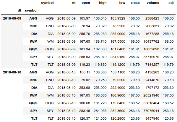
When working with price history, for convenient grouping and access to all data, the best solution is to use the multi-index (MultiIndex) with the date and tickers.
df = df.set_index(['dt', 'symbol'], drop=False).sort_index() df.tail(len(df.index.levels[1]) * 2) Using a multi-index, we can easily access the entire price history for all assets and can group an array separately by date and asset. We can also get a price history for one asset.
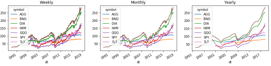
Here is an example of how you can easily group history by week, month, and year. And all this is shown on the graphs by Pandas:
# agg_rules = { 'dt': 'last', 'symbol': 'last', 'open': 'first', 'high': 'max', 'low': 'min', 'close': 'last', 'volume': 'sum', 'adj': 'last' } level_values = df.index.get_level_values # fig = plt.figure(figsize=(15, 3), facecolor='white') df.groupby([pd.Grouper(freq='W', level=0)] + [level_values(i) for i in [1]]).agg( agg_rules).set_index(['dt', 'symbol'], drop=False ).close.unstack(1).plot(ax=fig.add_subplot(131), title="Weekly") df.groupby([pd.Grouper(freq='M', level=0)] + [level_values(i) for i in [1]]).agg( agg_rules).set_index(['dt', 'symbol'], drop=False ).close.unstack(1).plot(ax=fig.add_subplot(132), title="Monthly") df.groupby([pd.Grouper(freq='Y', level=0)] + [level_values(i) for i in [1]]).agg( agg_rules).set_index(['dt', 'symbol'], drop=False ).close.unstack(1).plot(ax=fig.add_subplot(133), title="Yearly") plt.show() To correctly display the area with the chart legend, we move the index level with tickers to the second level above the columns using the Series (). Unstack (1) command. With DataFrame () this number will not work, but there is a solution below.
When grouping by standard periods, Pandas uses the latest calendar date of the group in the index, which is often different from actual dates. To fix this, update the index.
monthly = df.groupby([pd.Grouper(freq='M', level=0), level_values(1)]).agg(agg_rules) \ .set_index(['dt', 'symbol'], drop=False) An example of getting the price history of a certain asset (we take all the dates, the ticker QQQ and all the columns):
monthly.loc[(slice(None), ['QQQ']), :] # Monthly Asset Volatility
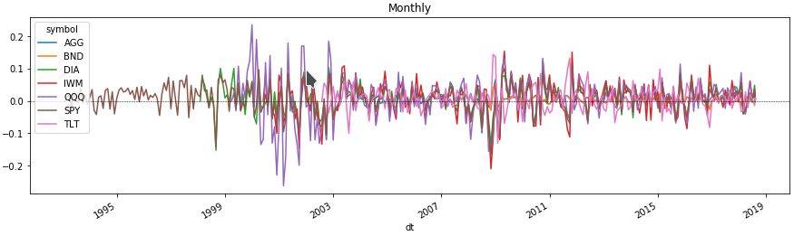
Now we can see in a few lines on the chart the change in the price of each asset for the period of interest to us. To do this, we get the percentage change in price, grouping the dataframe by the multi-index level with the asset ticker.
monthly = df.groupby([pd.Grouper(freq='M', level=0), level_values(1)]).agg( agg_rules).set_index(['dt', 'symbol'], drop=False) # . . monthly['pct_close'] = monthly.groupby(level=1)['close'].pct_change().fillna(0) # ax = monthly.pct_close.unstack(1).plot(title="Monthly", figsize=(15, 4)) ax.axhline(0, color='k', linestyle='--', lw=0.5) plt.show() Compare the return on assets
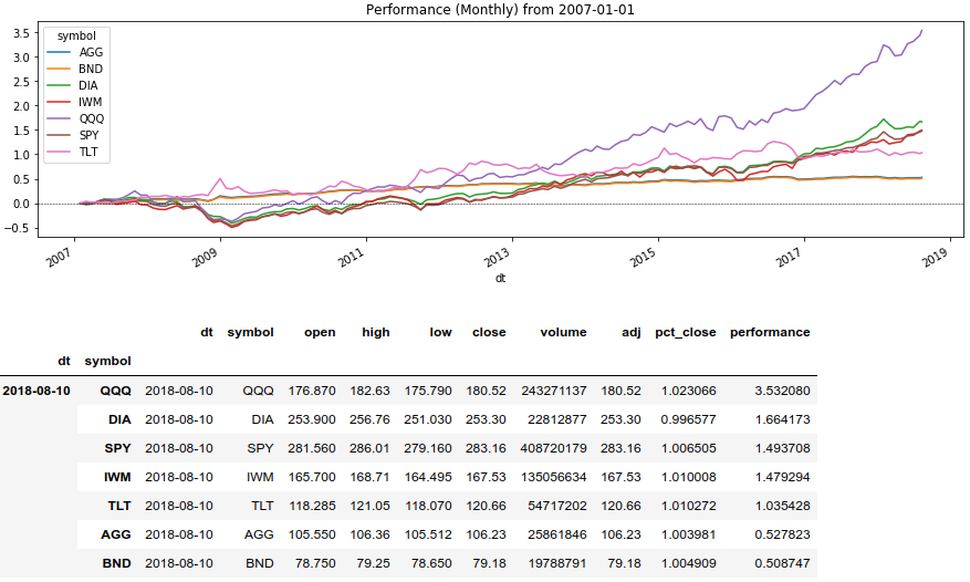
Now we use the Series (). Rolling () window method and derive the return on assets for a certain period:
Python code
rolling_prod = lambda x: x.rolling(len(x), min_periods=1).apply(np.prod) # monthly = df.groupby([pd.Grouper(freq='M', level=0), level_values(1)]).agg( agg_rules).set_index(['dt', 'symbol'], drop=False) # . . 1. monthly['pct_close'] = monthly.groupby(level=1)['close'].pct_change().fillna(0) + 1 # DataFrame 2007 fltr = monthly.dt >= '2007-01-01' test = monthly[fltr].copy().set_index(['dt', 'symbol'], drop=False) # dataframe test.loc[test.index.levels[0][0], 'pct_close'] = 1 # 1 # test['performance'] = test.groupby(level=1)['pct_close'].transform(rolling_prod) - 1 # ax = test.performance.unstack(1).plot(title="Performance (Monthly) from 2007-01-01", figsize=(15, 4)) ax.axhline(0, color='k', linestyle='--', lw=0.5) plt.show() # test.tail(len(test.index.levels[1])).sort_values('performance', ascending=False) Portfolio Rebalance Methods
So we got to the most delicious. In the examples, we will look at the results of the portfolio in the allocation of capital on pre-determined shares between several assets. And also we will add unique conditions according to which we will refuse some assets at the moment of capital distribution. If there are no suitable assets, we will assume that the capital lies with the broker in the cache.
In order to use the Pandas methods when rebalancing, we need to store the distribution shares and the rebalancing conditions in the DataFrame with grouped data. Now consider the rebalancing functions that will be passed to the DataFrame (). Apply () method:
Python code
def rebalance_simple(x): # data = x.unstack(1) return (data.pct_close * data['size']).sum() / data['size'].sum() def rebalance_sma(x): # , SMA50 > SMA200 data = x.unstack(1) fltr = data['sma50'] > data['sma200'] if not data[fltr]['size'].sum(): return 1 # , return (data[fltr].pct_close * data[fltr]['size']).sum() / data[fltr]['size'].sum() def rebalance_rsi(x): # , RSI100 > 50 data = x.unstack(1) fltr = data['rsi100'] > 50 if not data[fltr]['size'].sum(): return 1 # , return (data[fltr].pct_close * data[fltr]['size']).sum() / data[fltr]['size'].sum() def rebalance_custom(x, df=None): # data = x.unstack(1) for s in data.index: if data['dt'][s]: fltr_dt = df['dt'] < data['rebalance_dt'][s] # values = df[fltr_dt].loc[(slice(None), [s]), 'close'].values data.loc[s, 'custom'] = 0 # if len(values) > len(values[np.isnan(values)]): # RSI 100 data.loc[s, 'custom'] = talib.RSI(values, timeperiod=100)[-1] fltr = data['custom'] > 50 if not data[fltr]['size'].sum(): return 1 # , return (data[fltr].pct_close * data[fltr]['size']).sum() / data[fltr]['size'].sum() def drawdown(chg, is_max=False): # total = len(chg.index) rolling_max = chg.rolling(total, min_periods=1).max() daily_drawdown = chg/rolling_max - 1.0 if is_max: return daily_drawdown.rolling(total, min_periods=1).min() return daily_drawdown In order:
- rebalance_simple is the simplest function that will distribute the profitability of each asset by shares.
- rebalance_sma is a function that distributes capital to assets that have a 50-day moving average higher than the value for 200 days at the time of rebalancing.
- rebalance_rsi is a function that distributes capital to assets for which the value of the RSI indicator for 100 days is above 50.
- rebalance_custom is the slowest and most universal function, where we will calculate the indicator values from the daily price history of an asset at the time of rebalancing. Here you can use any conditions and data. Even download every time from external sources. But without a cycle can not do.
- drawdown - auxiliary function, showing the maximum drawdown of the portfolio.
In the rebalancing functions, we need an array of all the data on the date in terms of assets. The DataFrame (). Apply () method, by which we will calculate the results of the portfolios, will pass an array to our function, where the columns will become an index of rows. And if we make a multi-index, where tickers are zero, then a multi-index will come to us. We will be able to expand this multi-index into a two-dimensional array and get the data of the corresponding asset on each line.
Rebalancing portfolios
Now it’s enough to prepare the necessary conditions and make a calculation for each portfolio in a cycle. First of all, let's calculate the indicators on the daily price history:
# 1 , df['sma50'] = df.groupby(level=1)['close'].transform(lambda x: talib.SMA(x.values, timeperiod=50)).shift(1) df['sma200'] = df.groupby(level=1)['close'].transform(lambda x: talib.SMA(x.values, timeperiod=200)).shift(1) df['rsi100'] = df.groupby(level=1)['close'].transform(lambda x: talib.RSI(x.values, timeperiod=100)).shift(1) Now group the history under the desired rebalancing period using the methods described above. We will take in this case the values of the indicators at the beginning of the period, in order to exclude peeping into the future.
We describe the structure of portfolios and indicate the necessary rebalancing. Portfolios are calculated in a cycle, since we need to specify unique shares and conditions:
Python code
# : , , portfolios = [ {'symbols': [('SPY', 0.8), ('AGG', 0.2)], 'func': rebalance_sma, 'name': 'Portfolio 80/20 SMA50x200'}, {'symbols': [('SPY', 0.8), ('AGG', 0.2)], 'func': rebalance_rsi, 'name': 'Portfolio 80/20 RSI100>50'}, {'symbols': [('SPY', 0.8), ('AGG', 0.2)], 'func': partial(rebalance_custom, df=df), 'name': 'Portfolio 80/20 Custom'}, {'symbols': [('SPY', 0.8), ('AGG', 0.2)], 'func': rebalance_simple, 'name': 'Portfolio 80/20'}, {'symbols': [('SPY', 0.4), ('AGG', 0.6)], 'func': rebalance_simple, 'name': 'Portfolio 40/60'}, {'symbols': [('SPY', 0.2), ('AGG', 0.8)], 'func': rebalance_simple, 'name': 'Portfolio 20/80'}, {'symbols': [('DIA', 0.2), ('QQQ', 0.3), ('SPY', 0.2), ('IWM', 0.2), ('AGG', 0.1)], 'func': rebalance_simple, 'name': 'Portfolio DIA & QQQ & SPY & IWM & AGG'}, ] for p in portfolios: # rebalance['size'] = 0. for s, pct in p['symbols']: # rebalance.loc[(slice(None), [s]), 'size'] = pct # rebalance_perf = rebalance.stack().unstack([1, 2]).apply(p['func'], axis=1) # p['performance'] = (rebalance_perf.rolling(len(rebalance_perf), min_periods=1).apply(np.prod) - 1) # p['drawdown'] = drawdown(p['performance'] + 1, is_max=True) This time we will need to turn the trick with the indexes of columns and rows to get the desired multi-index in the rebalancing function. We achieve this by calling the DataFrame (). Stack (). Unstack ([1, 2]) methods in succession. This code will transfer the columns to the lower-order multi-index, and then return the multi-index back with tickers and columns in the desired order.
Ready portfolios for graphics
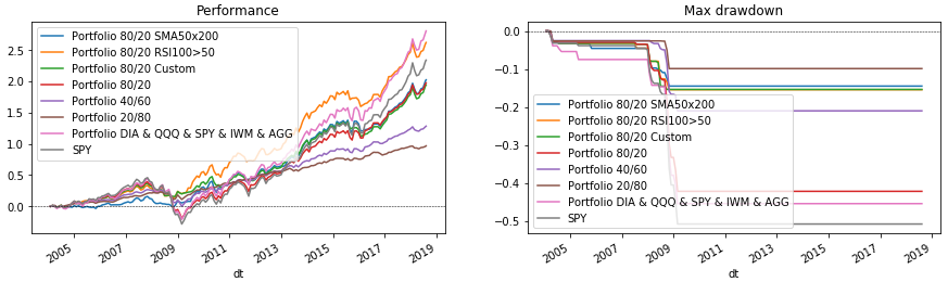
Now it remains to draw everything. To do this, once again run a cycle of portfolios, which will display data on the graphs. In the end we draw SPY as a benchmark for comparison.
Python code
fig = plt.figure(figsize=(15, 4), facecolor='white') ax_perf = fig.add_subplot(121) ax_dd = fig.add_subplot(122) for p in portfolios: p['performance'].rename(p['name']).plot(ax=ax_perf, legend=True, title='Performance') p['drawdown'].rename(p['name']).plot(ax=ax_dd, legend=True, title='Max drawdown') # print(f"{p['name']}: {p['performance'][-1]*100:.2f}% / {p['drawdown'][-1]*100:.2f}%") # SPY, rebalance.loc[(slice(None), ['SPY']), :].set_index('dt', drop=False).performance. \ rename('SPY').plot(ax=ax_perf, legend=True) drawdown(rebalance.loc[(slice(None), ['SPY']), :].set_index('dt', drop=False).performance + 1, is_max=True).rename('SPY').plot(ax=ax_dd, legend=True) ax_perf.axhline(0, color='k', linestyle='--', lw=0.5) ax_dd.axhline(0, color='k', linestyle='--', lw=0.5) plt.show() Conclusion
The considered code allows you to select different portfolio structures and rebalancing conditions. With it, you can quickly check whether, for example, it is worth holding gold (GLD) or emerging markets (EEM) in a portfolio. Try it yourself, add your own indicator conditions or select the parameters already described. (But remember the survivor’s mistake and that fitting to past data may not meet future expectations.) And after that, decide who you trust your portfolio to - Python or finco-sultant?
Repository: rebalance.portfolio
Source: https://habr.com/ru/post/419979/
All Articles