Early Universe 6. The Dynamics of a Homogeneous Expanding Universe, Part 2
On the website of free lectures MIT OpenCourseWare posted a course of lectures on cosmology by Alan Gus, one of the creators of the inflationary model of the universe.
Your attention is invited to the translation of the sixth lecture: "The dynamics of a homogeneous expanding universe, part 2".
Let's briefly repeat what we stopped at last time, because we have not finished the previous topic.
We considered an absolutely homogeneous universe in which matter fills the entire space. Recall that Newton came to the conclusion that such a system would be static. However, I argue that such a system will not be static even according to the laws of Newtonian mechanics.
')
I brought some evidence. For example, we considered the Gauss theorem for the law of Newton. With the help of fairly simple reasoning, we moved from the law of Newton, formulated as a force acting at a distance, to the law of Gauss. If the force of Newton's law is described by the law, then for any particle creating a gravitational field, the Gauss law is observed.
Gravitational acceleration vector flux v e c g through any closed surface is - 4 π G M where M - mass inside the surface. If we apply Gauss's law to the infinite distribution of matter, and assume that Newton was right and there are no gravitational forces, this would mean that the gravitational acceleration v e c g it would be zero everywhere. Then flow v e c g across any surface will also be zero. but - 4 π G M clearly not zero for any volume with a nonzero size containing a nonzero mass. Thus, such a formulation of the law of Newton clearly shows that the infinite distribution of matter cannot be static.
In addition, I showed another, more modern formulation of the law of Newton, the so-called Poisson equation. She was brought to those who are familiar with her. If you are not familiar with it, or anything terrible. It is not necessary.
For this formulation of the law of gravity, we introduce the gravitational potential φ, and we write the gravitational acceleration as a minus gradient φ. Then it can be shown that φ obeys the Poisson equation,
Again, it is immediately apparent that the static distribution of the substance is impossible. If the distribution of the substance was static, then the vector v e c g would be 0. This means that the gradient of φ would be equal to 0. This would mean that φ would be constant. If φ would be constant, ∇ 2 φ would be 0, and this is incompatible with the Poisson equation.
I also want to add that from a modern point of view, equations such as the Poisson equation are considered more fundamental than the original Newton equation, which considers gravity as an action at a distance. In particular, when generalizing Newton's law to the general theory of relativity, Einstein began with the Poisson equation, and not with a law describing force at a distance.
In the general theory of relativity there is no law describing the action of force at a distance. The general theory of relativity is formulated in a way very similar to the Poisson equation. The key idea underlying this approach is that all known laws of physics can be expressed locally.
The Poisson equation is a local equation. This is a differential equation that runs at every point in space and says nothing about how matter at one point in space affects matter at another point. This influence is a consequence of the equation, and is not built into the equation initially.
Then we discussed what would happen if we add up strength using Newton's law and action at a distance. I showed that we get a conditionally convergent integral. Such an integral converges, but it can converge to different values depending on the order in which the different parts of the integral are added.
We considered two possible order of addition forces. We calculated the force at the point P inside the infinite distribution of matter. We can assume that the whole picture is filled with substance. In our problem, matter uniformly fills the entire picture and the entire universe. The only thing we will do differently in our two calculations is to summarize the forces created by the substance in a different order.
If you take a substance ordered by concentric shells around P then each shell creates no force at the point P . Therefore, in the limit, when we add an infinite number of shells, the sum will still be equal to 0. Thus, for this case we get v e c g equal to 0.
But Newton's law does not tell us in what order the forces are added. Newton's law simply states that each mass creates a force proportional to 1 / r 2 and that is a vector. According to Newton, you need to add the force vectors created by each mass. Usually vector addition is commutative. It does not matter in which order we add them. But in our case, the order of addition matters. Therefore, the answer is ambiguous.
To see this, we consider a different order of addition. We will continue to use spherical shells because it’s easier to work with them. It could be folded in another way, but any other shape is much more difficult to use.
This time we will look at spherical shells, with a center at another point. We will call this point Q . We again calculate the force at the point P created by the infinite distribution of matter filling the space, that is, we solve the same problem as before, but we will add forces in a different order.
Last time, we showed that all matter inside a sphere, centered on Q and a radius less than the distance from Q before P giving contribution to the force at the point P . And the rest of the substance can be broken into spherical shells, for which the point P is inside. Inside the spherical shell, the force is zero. So all the rest of the substance does not make any contribution.
In this case, the force at the point P equal to the force created by a point mass located in Q , and a mass equal to the total mass of the shaded area. Obviously, this force is not zero. In addition, it is obvious that we can get any kind of force by choosing different points Q . We can increase strength by choosing a farther point. Since the force will always point in the direction of the point Q , we can get strength in any direction by choosing a point Q in the appropriate place.
Therefore, depending on how we sum up the strength, we can get any answer. Thus, the description of gravity as an action at a distance leads to ambiguity. The description of gravity in the form of Gauss's law or Poisson's law shows that the system cannot be static. Soon we will try to figure out exactly how it will behave.
Now I want to return to the argument that convinced Newton of the static nature of the universe. Newton believed that when calculating the gravitational acceleration at a certain point in the infinite distribution of matter, the problem of symmetry arises. All directions from this point look the same. If there is a gravitational acceleration at a given point, then where should it be directed? This symmetry argument is very logical and sounds very convincing. There can be no acceleration, simply because there is no preferred direction for it.
It would probably be difficult to convince Newton of the fallacy of this argument. I don't know if we could convince him or not. We do not have the opportunity to try to do it.
But if we had such an opportunity, we would try to explain to him that acceleration is usually measured in an inertial frame of reference. Newton himself always described it that way. For him, there was a unique inertial reference system, with an accuracy of constant speed, determined relative to fixed stars. This is Newton's terminology. So he defined the inertial frame of reference. All his laws of physics were valid in this inertial system.
On the other hand, if the entire space is filled with matter, which, as we say, will shrink, there are no fixed stars. The very idea of an inertial reference system disappears. There is no object that would be at rest or evenly moving relative to any potential inertial reference system.
In the absence of an inertial frame of reference, it must be recognized that all accelerations, like speeds, are relative. You can talk about the acceleration of one particle relative to another. But one cannot speak of the absolute acceleration of a particle, because there is no inertial reference system in which acceleration can be measured.
When all accelerations are relative, it turns out that the correct description, which we ultimately derive, is a description similar to the Hubble law. Hubble's law is the law of speeds. He says that from the point of view of any observer, all other objects are removed from this observer. Although it seems that the observer is in a special place, you can go to the reference system of any other observer and see exactly the same picture. Thus, the fact that all objects are removed from the observer does not violate uniformity. This does not violate the symmetry that we are trying to include in the system. The same applies to acceleration. I will not prove it now. We will show this in the course of our future calculations.
In our collapsing universe, any observer can consider himself to be at rest. Then the observer will see that all other particles are accelerated towards him. Although it sounds like the observer is in a special place, it is not. You can go to the reference system of any other observer and see that he is now at rest, and all other objects are accelerating towards him.
Now we are ready to go further and build a mathematical model that will show us how the uniform distribution of matter will behave. First we fix the problem of infinities. To do this, we start with a finite ball. Then, at the very end, we will increase the size of this ball to infinity.
Our goal is to build a mathematical model of our universe. We want to include three features that were previously discussed - isotropy, homogeneity, and the Hubble law. We will build it as a mechanical system, using the laws of mechanics known to us. We will use the laws of Newton. But I assure you that, although we will use Newton's laws, the answer we get will exactly match the answer given by general theory of relativity. Later we will discuss why this is so. We will not waste time on approximate calculations. We will receive an absolutely correct calculation, which will give us an absolutely correct answer.

In order to build a model of the universe, we imagine that our universe is a ball filled with substance of finite size. Let be t i - This is the initial time in our picture. This moment of time does not have to be any special, in terms of the evolution of the universe. When we build a model, we can calculate how the universe will behave in later times than t i and in times earlier than t i . t i - this is just the current time.
For a time t i we will give our ball the maximum size R m a x , i . I called it maximal because the ball is filled with particles. Thus, this is the initial maximum distance from the center of the ball to any particle. The initial is meant during t i . We will consider the substance filling the ball as dust from very small particles. The substance has a density ρ i . The substance is uniform and isotropic, at least isotropic from the center.
Now we want to add the Hubble law. Let us have all the matter, in our model universe, expanding, and expanding exactly according to the Hubble law. Namely, all speeds will be directed from the center with a value proportional to the distance. I will denote the particle velocity v i , i means initial speed. For any particle at the initial time, the speed will obey the Hubble law. It will be equal to some constant, which I will call H i - the initial value of the Hubble constant multiplied by the vector v e c r which is equal to the vector from the center of the ball to the particle. It shows where the particle in question is.
In this way, v e c v i - the initial velocity of any particle. H i - Hubble's initial constant. BUT v e c r - particle position.
As I said, we will start with a finite-sized system with which we can work. We know how to unequivocally calculate, at least in principle, how such a system will evolve under given initial conditions. At the end of the calculation we will move to the limit when R m a x , i tends to infinity. In this way, we will extend our model to infinite space.
I also want to say a few words about infinity, since I recently met with one interesting thing. This is a small digression, you can ignore it. But for those who are interested, the concept of infinity presented an unexpected surprise when considering the multiverse, which I talked about a little in the review lecture, and to which we will return at the end of the course.
The multiverse made it work with infinities much more carefully than before. In the process, I learned some things about infinity that surprised me. Basically, in physics, we consider infinity as the limit of finite systems, as we do in our model. If we want to understand the behavior of an infinite system, in physics we very often begin by considering a finite system, with which it is much easier to work mathematically. Then we take the limit at which the system gets bigger and bigger.
In physics, it works in almost all situations. I believe this works because we assume that physical interactions are local. What happens very far does not affect what is happening here.
As we make our sphere more and more, we add matter at greater and greater distances. This new substance that we add will not greatly influence what is going on inside. In fact, in our problem, the additional substance added from the outside will have no influence on what is going on inside, due to the fact that the gravitational field inside the spherical shell is 0.
This is a typical situation, and because of this, physicists are always inclined to regard infinity as the limits of finite systems. However, I want to point out that this is not always correct. There are times when this is absolutely wrong. Mathematicians are aware of this, but physics is usually not.
Therefore, I want to note that not all infinities are well described as the limits of finite systems. This does not apply to the description of our model universe. Here we are fine. We will continue the discussion of our model after I finish my small digression.
As an example of a system that is infinite and not very well described as the limit of finite systems, one can take a lot of natural numbers m a t h b b N .
Suppose we want to describe the set of natural numbers as the limit of a finite set. You can try to consider the set of all natural numbers as a set of natural numbers less than N with N tending to infinity. If we take sets of more and more numbers and take the limit, do we get the set of all natural numbers?
You might think that the answer is yes. I argue that the resulting set is not equal to the set of integers. In fact, I argue that the limit does not exist at all, so it cannot be equal to the set of integers.
To clarify this, I remind you what the limit is. Since we do not have a mathematical course, I will not give a strict definition. I'll just give you an example that will refresh the facts that you learned in math courses.
Suppose we are considering the limit sin(x)/x at x tending to 0. It is known what it is equal to. Usually use the rule of L'Hôpital. But you can just directly use the definition of the limit. The limit value is 1.
For anyone x not equal to 0, we can evaluate this expression. With x=0 expression is ambiguous. As x getting closer and closer to 0, the resulting numbers are getting closer to 1. We can get the number arbitrarily close to 1 by choosing x close enough to 0.
If we apply the same concept to the set of integers from 1 to N, will it approach the set of all natural numbers with increasing N? Are numbers from 1 to 10 close to the set of all natural numbers? Not. And from 1 to a million? Still infinitely far. From 1 to billion? From 1 to 10 to the hundredth?
No matter what number we choose as the upper limit, we are still infinitely far from the set of natural numbers. We are not getting closer. Our sets do not converge to the set of natural numbers. This is a different concept.
What does it matter? Are there any questions, where it is important, do you consider natural numbers determined by any other means or this limit? Let's first say how they are defined.
If you ask mathematicians how they define a set of natural numbers, I think they will all say that they use Peano's axioms. The key point in Peano's axioms, which determines the existence of an infinite number of natural numbers, is the axiom of succession.
One of Peano's axioms, which mathematically describe natural numbers, is the statement that each natural number has a number following it. In addition, there are other statements that ensure that the next number is not one of the previous ones. Thus, for any number, there is an even greater number. This set of axioms initially guarantees the infinity of the set of natural numbers. It is not considered as the limit of finite sets and cannot be considered as the limit of finite sets. Because no finite set is like an infinite set.
Does it matter? Are there any tasks in which it is important, can we describe whole numbers in this way or not? I recognize that the tasks that I know sound far-fetched. But I want to say that in mathematics the word "contrived" does not matter.If you find a contradiction somewhere, no one will tell you that this contradiction should be ignored, because it is contrived. If this is really a contradiction, it matters.
The question in which it really matters is whether we consider natural numbers as initially infinite, or we consider them as a limit, for example, the question is - what part of natural numbers is so large that when doubling, they cease to be natural numbers?
If we consider a finite set, for any N, no matter how large N is, half of the integers from this set are so large that they cannot be doubled, so that they remain in this set. This relationship will be fulfilled no matter how large we chose N.
On the other hand, if we look at an infinite series of natural numbers, we know that any natural number can be doubled, we just get another natural number. This is an example of the property of natural numbers, which will be wrong if we take the set of natural numbers as the limit. So you can not do.
It was a small digression. This is just a warning that you need to be careful about infinity as the limit of finite sets. However, it is not directly related to our topic.
Note on the form used.
Let's go back to our model. I also want to make a couple of comments on the form used in the model. We use spheres. You may ask why spheres?
The sphere is by far the simplest form with which we can work. The sphere also guarantees isotropy, at least isotropy from the center. We could, having done much more work, use, for example, a cube, increasing the cube more and more. As the cube gets bigger and bigger, it will also fill the entire space. It can be assumed that this other method will give the same answer. And indeed it is.
If we used cubes, we would have much more computation. But we would get the same answer. The cube is quite symmetrical. In this case, he will give the same result as the sphere. I will not tell you how to calculate the result for an arbitrary form. But I guarantee that the cube will give the same answer.
On the other hand, if we use parallelepipeds, with three, or at least two different sides, we will start with an initially asymmetric shape. One of the directions will be highlighted. Then, if we use such parallelepipeds, in the same way as we use spheres, we will initially create anisotropy. We get an anisotropic model of the universe.
As we try to model the real universe, which is highly isotropic, we use a form that guarantees isotropy. A sphere is the simplest form you can use.
Now, let's add dynamics to our model. The dynamics we add will be purely Newtonian dynamics. We will consider a substance that fills a sphere as dust of Newtonian particles, or, if you prefer, as a gas of Newtonian particles.
These particles will be non-relativistic, which is meant by the word Newtonian. This model describes our real universe for a significant segment of its evolution, but not for the entire period of evolution. Before we continue, I want to say a few words about the real universe and what kind of matter dominated it in different epochs of evolution.
At the beginning in our universe, we believe that radiation dominated. This means that, if we trace the evolution of our universe back in time, and see what happened in ever earlier times, the photons of the cosmic background radiation will experience a blue shift.
We found out that they are experiencing a redshift as the universe expands. This means that if we extrapolate in the opposite direction, they will experience a blue shift. Each photon is becoming more energetic. The number of photons remains constant. Their concentration increases due to a decrease in volume. And they are becoming more energetic.
Meanwhile, the concentration of particles of ordinary matter and dark matter, from whatever it was, also increases when moving backward in time. But they do not become more energetic. The proton remains a particle whose energy is equal to the mass of the proton multiplied byc 2 .
Thus, as it moves backward in time, the energy density of the cosmic microwave background radiation becomes more and more compared to the energy density of a substance. Later we will learn how to accurately calculate it. They are compared at the age of the universe about 50,000 years.
STUDENT: If particles are waves, then why don't they change?
TEACHER: Actually, they change a little. But we assume that these particles have negligible speed. Their momentum is experiencing a blue shift. But the blue offset is proportional to the initial value. If the initial value is very small, even when it shifts to a higher direction, the momentum still remains insignificant.
Thus, in the real universe, up to about 50,000 years, radiation dominated. We will talk about this in a few lectures. But today we do not take this into account. Then, from about 50,000 years to 9 billion years, a fairly long period in the history of the universe, matter dominated the universe. Substance means non-relativistic substance. This is a standard term in cosmology. When we say that matter dominates in the universe, although we do not use the word non-relativistic, this is implied by all. This is a case that we will consider today, the usual non-relativistic substance filling the space.
Then another change occurred in our real universe - from about 9 billion years to the present, and, presumably, there will also be in the future, dark energy has become dominant in the universe. Dark energy is something that causes the universe to expand rapidly. The universe is expanding rapidly from about 9 billion years after the Big Bang.
Ordinary matter does not turn into dark energy, as one would assume due to a change in dominance. They just behave differently when the universe expands. The density of ordinary matter decreases in proportion to the cube of the scale factor. A fixed number of particles is distributed over an ever increasing volume. Dark energy, for reasons that we learn about towards the end of the course, does not change its energy density as the universe expands. 9 billion years ago, the density of ordinary matter fell below the density of dark energy. Then the dark energy began to dominate and the universe began to expand rapidly. Today, dark energy accounts for about 60% or 70% of total energy. This is not absolute dominance. But this is the biggest part.
For today's calculation, we will focus on the middle period and pretend that this is the whole story. We will come back and discuss other eras. We will not ignore them. But today we will not discuss them.
So, we consider the universe in which substance dominates. We will use Newtonian mechanics. Despite the fact that we will use Newtonian mechanics, I assure you, and later I will try to give some arguments, it will give the exact same answer as the general theory of relativity.
In order to write down the equations describing the expansion of the ball, we will use spherical shells. We will present our ball in the form of its shells. In other words, at the initial moment of time we divide the substance into shells. We will enter a designation for each of the shells and trace their evolution.
The reason why we can describe all matter using shells is that the initial velocities of all particles are directed along the radius. According to the Hubble law, the speeds are proportional to the radius vector, deferred from the center of the ball. Therefore, all our initial velocities are directed along the radius.
In addition, Newtonian gravity for particles will also be directed along the radius. Therefore, the movement of any particle will be directed along the radius. There will never be any forces that act on a particle in the tangential direction, where tangential means any direction other than the radial one. When the radius of each particle changes, its angular variables ϑ and ϕ will be constant in time. Therefore, I will no longer talk about them.
Each shell has a designationr i equal to its radius at the initial moment of timet i .In the future, this designation of the shell is preserved.
To describe the movement we introduce the functionr ( r i , t ) . The function is equal to the shell radius r i at the moment of time t . Function r ( r i , t ) shows us where the shell is at any later or earlier time.I must say that in the textbook you will see a simpler conclusion than the one that I will show you. Why do I complicate it? The fact is that my calculation will show more than the one given in the textbook. In most textbooks, it is assumed that the movement of the shells will continue to obey the Hubble law and maintain a completely uniform density. We will not assume that the substance remains homogeneous. We will prove that it remains homogeneous. It seems to me that it is much better to prove something than to simply assume without proving it.
There is another problem that is a bit more complicated. Again, this is a subtlety that is most likely not mentioned in textbooks. We have various expanding shells. We can calculate the force acting on any shell, if we know what substance is inside this shell. Shells outside do not create strength. Therefore, it is very important to know in which order the shells are located. Initially, of course, we know that. They are ordered according tor i .But as soon as they begin to move, in principle, there is a possibility that the shells will begin to cross each other.
If the shells intersect, our equations of motion will change, because the amount of substance acting on the shell will change. We will have to take this into account. Fortunately, this problem does not arise. We show it as follows. Initially, all shells are removed from each other according to the Hubble law. Hubble's law says that any two particles move away from each other with a relative speed proportional to their distance. This is true for any two shells. If the shells begin to intersect, they definitely won't do it right away. There are no two shells that are initially close to each other. All shells initially move away from each other.
This situation may change due to operating forces. However, we can write down the equations that will be executed, at least until intersections of the shells appear. If the shells intersect, these equations should be valid up to the time of the intersection of the shells. Therefore, the equations must show that the shells will intersect. Shells cannot begin to intersect against the equations of motion. We will see that according to our equations, there will be no intersections of the shells.
So, we write the equations that will be valid until there are no intersections of the shells. While there are no intersections of the shells, the total mass inside any shell does not depend on time. These are just other shells inside. Thus, on the shell with the initial radiusr i , the force generated by the mass inside the shell. We can write a formula for the mass inside the shell. The mass inside the shell with an initial radiusr i is equal to the initial volume of the shell multiplied by the initial mass density,ρ i
We compose a differential equation
Newton's law determines the acceleration of an arbitrary particle in our system. Newton's law states that the acceleration is directed in the opposite direction from the unit radius vector to the particle and is equal to Newton's constant multiplied by the mass inside the sphere divided by the square of the distance of the shell from the origin. This distance is equal to the functionr ( r i , t ) . This is the shell radius at a particular point in time.
This is true for any shell denoted by a variable. r i .
This is a really important equation. Everything else follows from it. It reflects Newton's theorem, that if the mass is spherically symmetric distributed, then the mass of any shell of a larger radius than the distance to the particle does not contribute to the acceleration of the particle. Acceleration is determined only by the mass of shells of smaller radii.
We know that all movements occur along radii. All we need is to find out how.r changes with time. We can write this as a conventional differential equation forr , without any vectors.
¨ r is acceleration. We setM ( r i ) from the previous formula.r is a function ofr i and t .I will not indicate this anymore.
When expanding the systemr i is just a constant, different for each shell, but constant over time. Imagine that we are solving a problem for a specific shell.ρ i is also a constant. It is equal to the density at the initial moment of time and retains its value. We have obtained a differential equation in which only time changes
r , and nothing else. This is a second order differential equation forr .
There is one thing that you must all remember when working with second-order differential equations. In order to have a single solution, we need initial conditions. If this is a second-order equation, and these are usually Newton's equations, we must indicate the initial position and the initial velocity so that the second-order equation gives a unique answer.
We will set the initial position valuer and initial velocity˙ r particles. We will have a system that we can give to math. If the mathematician is smart enough, he can solve it. So we want to set the initial value
r , initial means at timet i . Obviously, it is just equal r i .
If we want to have a unique solution for this equation, then we also need to set the initial velocity value. ˙ r . Initial again means during t i .It is determined by the Hubble constant. Each initial particle velocity is equal to the initial value of the Hubble constant multiplied by the radius.
This is the Hubble expansion that we initially introduced into the system. We have a purely mathematical system. We have a second-order differential equation and initial conditions forr and ˙ r .It gives a unique solution. This is pure mathematics. No more physics is needed, at least at this stage.
You can see interesting mathematical features of this system of equations. We will see that these equations miraculously preserve the homogeneity of our system. This is built into the equations. The key feature of these equations is that you can get rid ofr i by changing the variables. Let's define a new function.
u . I arbitrarily chose a letter to designate, you can take whatever you like.
For any function r ( r i , t ) you can always define a new function that is equal to the original function divided byr i .
Now let's see what happens with our equations. I affirm thatr i will disappear. Let's see how this happens:
From the equation you can see how the reduction occurs r i . r i in the cube in the numerator is proportional to the volume of the sphere. In the denominatorr i stands also in the cube. One r i appeared due to the change of variables,r 2 i appeared due to inverse square law. Thus, the reduction
r i appears if the force decreases as1 / r 2 . If the force declined according to another law, if it was only slightly different from 1 / r 2 , thenr i would not be reduced in the formula. Exactly the abbreviationr i is crucial to ensure homogeneity in the evolution of the system. If, according to Newton, force decreases, as1 / r 2 squared, the system remains homogeneous. Otherwise, no. This is a very interesting fact.
So, r i have decreased. Now we get a simple equation for d d o t u more without r i in the equation. It means that u gives a solution for any r i . We no longer have different solutions for different values. r i . r i disappears from the task. We have the only solution independent ofr i . It is true for all r i .
What did I forget to mention? Initial conditions. To get a single solution, we must have not only a differential equation independent ofr i . We will not have a single solution if we do not verify the initial conditions, which should also not depend on r i .And they do not depend.
Initial valueu ( r i , t i ) is equal to the initial valuer divided byr i . But the initial value r equally r i . For anyone r i we get:
Now consider the initial value ˙ u . It is equal to
If you look closely, you can understand the physical interpretation of the value u . u is nothing more than a large-scale factor that we talked about earlier. We proved that we had a uniformly expanding system. Initially, we had a homogeneous expansion, but we did not know until we considered the equation of motion whether the universe would continue to expand uniformly. However it is. This means that the extension can be described using a scale factor. We found out that
u is completely determined by equations that do notr i . In this way, u does not depend onr i and can be considered as just a function of timet . We can also change its name to a ( t ) to establish identity with a scale factor:
It also shows that
What does this mean? r i is a companion coordinate. We tagged each shell according to its starting position.r i . As you expand, for each shell label r i saved. It marks particles no matter where they move. BUT r is the physical distance, in this case from the origin, equal to the scale factor multiplied by the accompanying distance. These equations are useful to write in another form. The previous differential equation used
ρ i . This is very convenient because ρ i is a constant. It does not change with time. However, it is also useful to write a differential equation using the valueρ , which changes over time to see the relationship between physical quantities at a given point in time. This is not hard to do, because we know what the density is at any given time. For any shell, we can calculate the density as the total mass inside the shell divided by volume. We know that the density remains homogeneous, since with us all distances are simply proportional to the total scale factor. Therefore, the density will be uniform. We can calculate the density inside the shell by taking
M ( r i ) , for which we already have a formula, and which does not depend on time, and dividing it by the volume inside the shell.
This is the expected result. The density is equal to the original density divided by the cube of the scale factor. The scale factor is 1 at the initial time, according to our definitions. Thus, in the equation we get the ratio of scale factors in the cube. As the universe expands, the density falls inversely with the scale factor in the cube.
Now we can rewrite the equation for¨ a , using the current mass density.
This equation gives the deceleration of our model universe, depending on the current mass density. Note that it really depends only on the mass density. It defines the relationship¨ a /a . So it should be, because we recall that a is measured in divisions per meter. At the same time divisions are reduced. We get the answer in physical units. I said at the beginning that when we finish, we will take the limit when the initial maximum radius
R m a x , i goes to infinity.R m a x , i does not appear in any of these equations. Therefore, when strivingR m a x , i to infinity, in fact, nothing is happening. This means that the answer we received does not depend on how big the ball is, if everything we consider is inside the ball. Adding additional substance from the outside does not change anything. So in the limit, we add an infinite amount of matter outside. To go to the limitR m a x , i tending to infinity, there is no need to do anything. Ultimately, we want to get different solutions to this equation and understand how they look. Today I want to take another step in this direction, rewriting the equation a little differently, which will help us figure out what the solutions look like. I want to find the first integral of this equation.
To find the first integral, I want to go back to the equation where I use ρ i , notρ ( t ) . Its advantage is that ρ i does not depend on time. Have ρ has its own dependence on time, which I do not want to take into account now. Therefore, if I use the formula in which is usedρ i , dependence on time will be only for the scale factor. I use the previous equation, but I will replace
u on a because we renamedu at a .I will also transfer all members to one side. Turns out
This is a second-order differential equation, which is very often found in Newtonian mechanics, this equation determines ¨ a , accelerationa , through valuesa .
In Newtonian mechanics it is often possible to use the law of conservation of energy. In this case, I do not know whether to call it energy conservation. Later we will talk about the physical meaning of the result we obtained. But, of course, as a mathematical technique, we can use the same method that is used in Newtonian mechanics to obtain the law of conservation of energy.
To obtain the energy conservation law corresponding to this equation, we multiply the equation by the integrating factor,˙ a .After that, the whole expression will be a complete derivative. This equation is equivalent to
This can be easily verified. If I differentiateE , I get exactly this equation. So they are equivalent. In this way,E is a conserved value. Now, if we want to tie
E with any energy, there are different ways to do it. One way is to multiplyE on m r 2 i and consider this as the energy of the test particle on the surface of the sphere.m is the mass of the test particle.r i is the initial radius of the test particle. In this way
E p h i s , or the physical energy of the hypothetical test particle will be equal to
If we consider that for a test particle r i isR m a x , i , that is, we are talking about the boundary of our sphere, then it is clear that it remains here. It turns out the kinetic energy plus potential energy - where the potential energy is negative - of a point particle at the boundary of the sphere. If we want to apply this equation to a particle inside a sphere, it will be a little more difficult to find the correct interpretation. If the particle is inside the sphere, if
r i is not equal to the maximum radius of the sphere, thenE p h i s , in fact, is not the potential energy of the particle.To calculate the potential energy of a particle, it is necessary to calculate what work will have to be done in order to take a particle at infinity and place it in its place. This takes into account the contribution of the mass inside the sphere on which the particle is located, which determines the force at this point. But we also have a contribution from a substance outside the sphere with the particle.When calculating the potential energy, I just don't get
G m multiplied by the mass inside the sphere divided by the distance from the center. I will get a much more complex expression. In fact, the energy I receive is not saved. Why is it not saved?It is not preserved, because in the presence of moving masses there is no reason for its preservation. The energy of a point particle moving in a field of static masses is conserved. This is what you know from the relevant courses. If other particles move, then the total energy of the entire system is conserved. But the potential energy of a particular particle moving in the gravitational field of other particles may not be saved.In addition to the particle energy at the boundary, the total energy of the system is also conserved. She will be associated with
E another constant of proportionality and will persist for an obvious reason. Here you need to be careful to understand what is saved, why and how to use it.
Your attention is invited to the translation of the sixth lecture: "The dynamics of a homogeneous expanding universe, part 2".
The impossibility of the existence of a static universe
Let's briefly repeat what we stopped at last time, because we have not finished the previous topic.
We considered an absolutely homogeneous universe in which matter fills the entire space. Recall that Newton came to the conclusion that such a system would be static. However, I argue that such a system will not be static even according to the laws of Newtonian mechanics.
')
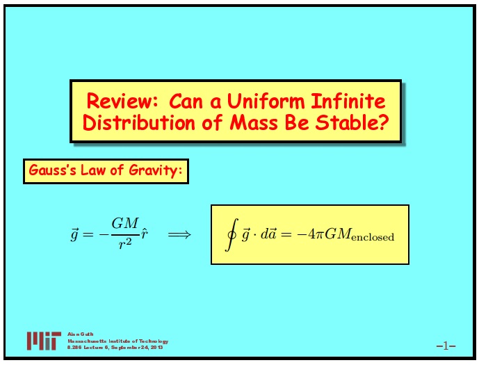
I brought some evidence. For example, we considered the Gauss theorem for the law of Newton. With the help of fairly simple reasoning, we moved from the law of Newton, formulated as a force acting at a distance, to the law of Gauss. If the force of Newton's law is described by the law, then for any particle creating a gravitational field, the Gauss law is observed.
Gravitational acceleration vector flux v e c g through any closed surface is - 4 π G M where M - mass inside the surface. If we apply Gauss's law to the infinite distribution of matter, and assume that Newton was right and there are no gravitational forces, this would mean that the gravitational acceleration v e c g it would be zero everywhere. Then flow v e c g across any surface will also be zero. but - 4 π G M clearly not zero for any volume with a nonzero size containing a nonzero mass. Thus, such a formulation of the law of Newton clearly shows that the infinite distribution of matter cannot be static.
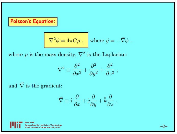
In addition, I showed another, more modern formulation of the law of Newton, the so-called Poisson equation. She was brought to those who are familiar with her. If you are not familiar with it, or anything terrible. It is not necessary.
For this formulation of the law of gravity, we introduce the gravitational potential φ, and we write the gravitational acceleration as a minus gradient φ. Then it can be shown that φ obeys the Poisson equation,
$$ display $$ ∇ ^ 2φ = 4πGρ $$ display $$
where ρ is the mass density.Again, it is immediately apparent that the static distribution of the substance is impossible. If the distribution of the substance was static, then the vector v e c g would be 0. This means that the gradient of φ would be equal to 0. This would mean that φ would be constant. If φ would be constant, ∇ 2 φ would be 0, and this is incompatible with the Poisson equation.
I also want to add that from a modern point of view, equations such as the Poisson equation are considered more fundamental than the original Newton equation, which considers gravity as an action at a distance. In particular, when generalizing Newton's law to the general theory of relativity, Einstein began with the Poisson equation, and not with a law describing force at a distance.
In the general theory of relativity there is no law describing the action of force at a distance. The general theory of relativity is formulated in a way very similar to the Poisson equation. The key idea underlying this approach is that all known laws of physics can be expressed locally.
The Poisson equation is a local equation. This is a differential equation that runs at every point in space and says nothing about how matter at one point in space affects matter at another point. This influence is a consequence of the equation, and is not built into the equation initially.
Ambiguity of gravitational acceleration calculation
Then we discussed what would happen if we add up strength using Newton's law and action at a distance. I showed that we get a conditionally convergent integral. Such an integral converges, but it can converge to different values depending on the order in which the different parts of the integral are added.
We considered two possible order of addition forces. We calculated the force at the point P inside the infinite distribution of matter. We can assume that the whole picture is filled with substance. In our problem, matter uniformly fills the entire picture and the entire universe. The only thing we will do differently in our two calculations is to summarize the forces created by the substance in a different order.
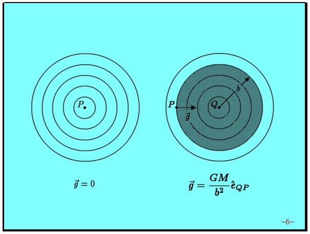
If you take a substance ordered by concentric shells around P then each shell creates no force at the point P . Therefore, in the limit, when we add an infinite number of shells, the sum will still be equal to 0. Thus, for this case we get v e c g equal to 0.
But Newton's law does not tell us in what order the forces are added. Newton's law simply states that each mass creates a force proportional to 1 / r 2 and that is a vector. According to Newton, you need to add the force vectors created by each mass. Usually vector addition is commutative. It does not matter in which order we add them. But in our case, the order of addition matters. Therefore, the answer is ambiguous.
To see this, we consider a different order of addition. We will continue to use spherical shells because it’s easier to work with them. It could be folded in another way, but any other shape is much more difficult to use.
This time we will look at spherical shells, with a center at another point. We will call this point Q . We again calculate the force at the point P created by the infinite distribution of matter filling the space, that is, we solve the same problem as before, but we will add forces in a different order.
Last time, we showed that all matter inside a sphere, centered on Q and a radius less than the distance from Q before P giving contribution to the force at the point P . And the rest of the substance can be broken into spherical shells, for which the point P is inside. Inside the spherical shell, the force is zero. So all the rest of the substance does not make any contribution.
In this case, the force at the point P equal to the force created by a point mass located in Q , and a mass equal to the total mass of the shaded area. Obviously, this force is not zero. In addition, it is obvious that we can get any kind of force by choosing different points Q . We can increase strength by choosing a farther point. Since the force will always point in the direction of the point Q , we can get strength in any direction by choosing a point Q in the appropriate place.
Therefore, depending on how we sum up the strength, we can get any answer. Thus, the description of gravity as an action at a distance leads to ambiguity. The description of gravity in the form of Gauss's law or Poisson's law shows that the system cannot be static. Soon we will try to figure out exactly how it will behave.
Symmetry problem
Now I want to return to the argument that convinced Newton of the static nature of the universe. Newton believed that when calculating the gravitational acceleration at a certain point in the infinite distribution of matter, the problem of symmetry arises. All directions from this point look the same. If there is a gravitational acceleration at a given point, then where should it be directed? This symmetry argument is very logical and sounds very convincing. There can be no acceleration, simply because there is no preferred direction for it.
It would probably be difficult to convince Newton of the fallacy of this argument. I don't know if we could convince him or not. We do not have the opportunity to try to do it.
But if we had such an opportunity, we would try to explain to him that acceleration is usually measured in an inertial frame of reference. Newton himself always described it that way. For him, there was a unique inertial reference system, with an accuracy of constant speed, determined relative to fixed stars. This is Newton's terminology. So he defined the inertial frame of reference. All his laws of physics were valid in this inertial system.
On the other hand, if the entire space is filled with matter, which, as we say, will shrink, there are no fixed stars. The very idea of an inertial reference system disappears. There is no object that would be at rest or evenly moving relative to any potential inertial reference system.
In the absence of an inertial frame of reference, it must be recognized that all accelerations, like speeds, are relative. You can talk about the acceleration of one particle relative to another. But one cannot speak of the absolute acceleration of a particle, because there is no inertial reference system in which acceleration can be measured.
When all accelerations are relative, it turns out that the correct description, which we ultimately derive, is a description similar to the Hubble law. Hubble's law is the law of speeds. He says that from the point of view of any observer, all other objects are removed from this observer. Although it seems that the observer is in a special place, you can go to the reference system of any other observer and see exactly the same picture. Thus, the fact that all objects are removed from the observer does not violate uniformity. This does not violate the symmetry that we are trying to include in the system. The same applies to acceleration. I will not prove it now. We will show this in the course of our future calculations.
In our collapsing universe, any observer can consider himself to be at rest. Then the observer will see that all other particles are accelerated towards him. Although it sounds like the observer is in a special place, it is not. You can go to the reference system of any other observer and see that he is now at rest, and all other objects are accelerating towards him.
Mathematical model of the universe
Now we are ready to go further and build a mathematical model that will show us how the uniform distribution of matter will behave. First we fix the problem of infinities. To do this, we start with a finite ball. Then, at the very end, we will increase the size of this ball to infinity.
Our goal is to build a mathematical model of our universe. We want to include three features that were previously discussed - isotropy, homogeneity, and the Hubble law. We will build it as a mechanical system, using the laws of mechanics known to us. We will use the laws of Newton. But I assure you that, although we will use Newton's laws, the answer we get will exactly match the answer given by general theory of relativity. Later we will discuss why this is so. We will not waste time on approximate calculations. We will receive an absolutely correct calculation, which will give us an absolutely correct answer.
In order to build a model of the universe, we imagine that our universe is a ball filled with substance of finite size. Let be t i - This is the initial time in our picture. This moment of time does not have to be any special, in terms of the evolution of the universe. When we build a model, we can calculate how the universe will behave in later times than t i and in times earlier than t i . t i - this is just the current time.
For a time t i we will give our ball the maximum size R m a x , i . I called it maximal because the ball is filled with particles. Thus, this is the initial maximum distance from the center of the ball to any particle. The initial is meant during t i . We will consider the substance filling the ball as dust from very small particles. The substance has a density ρ i . The substance is uniform and isotropic, at least isotropic from the center.
Now we want to add the Hubble law. Let us have all the matter, in our model universe, expanding, and expanding exactly according to the Hubble law. Namely, all speeds will be directed from the center with a value proportional to the distance. I will denote the particle velocity v i , i means initial speed. For any particle at the initial time, the speed will obey the Hubble law. It will be equal to some constant, which I will call H i - the initial value of the Hubble constant multiplied by the vector v e c r which is equal to the vector from the center of the ball to the particle. It shows where the particle in question is.
v e c v i = H i c d o t v e c r
In this way, v e c v i - the initial velocity of any particle. H i - Hubble's initial constant. BUT v e c r - particle position.
As I said, we will start with a finite-sized system with which we can work. We know how to unequivocally calculate, at least in principle, how such a system will evolve under given initial conditions. At the end of the calculation we will move to the limit when R m a x , i tends to infinity. In this way, we will extend our model to infinite space.
A small digression about infinities
I also want to say a few words about infinity, since I recently met with one interesting thing. This is a small digression, you can ignore it. But for those who are interested, the concept of infinity presented an unexpected surprise when considering the multiverse, which I talked about a little in the review lecture, and to which we will return at the end of the course.
The multiverse made it work with infinities much more carefully than before. In the process, I learned some things about infinity that surprised me. Basically, in physics, we consider infinity as the limit of finite systems, as we do in our model. If we want to understand the behavior of an infinite system, in physics we very often begin by considering a finite system, with which it is much easier to work mathematically. Then we take the limit at which the system gets bigger and bigger.
In physics, it works in almost all situations. I believe this works because we assume that physical interactions are local. What happens very far does not affect what is happening here.
As we make our sphere more and more, we add matter at greater and greater distances. This new substance that we add will not greatly influence what is going on inside. In fact, in our problem, the additional substance added from the outside will have no influence on what is going on inside, due to the fact that the gravitational field inside the spherical shell is 0.
This is a typical situation, and because of this, physicists are always inclined to regard infinity as the limits of finite systems. However, I want to point out that this is not always correct. There are times when this is absolutely wrong. Mathematicians are aware of this, but physics is usually not.
Therefore, I want to note that not all infinities are well described as the limits of finite systems. This does not apply to the description of our model universe. Here we are fine. We will continue the discussion of our model after I finish my small digression.
As an example of a system that is infinite and not very well described as the limit of finite systems, one can take a lot of natural numbers m a t h b b N .
Suppose we want to describe the set of natural numbers as the limit of a finite set. You can try to consider the set of all natural numbers as a set of natural numbers less than N with N tending to infinity. If we take sets of more and more numbers and take the limit, do we get the set of all natural numbers?
You might think that the answer is yes. I argue that the resulting set is not equal to the set of integers. In fact, I argue that the limit does not exist at all, so it cannot be equal to the set of integers.
To clarify this, I remind you what the limit is. Since we do not have a mathematical course, I will not give a strict definition. I'll just give you an example that will refresh the facts that you learned in math courses.
Suppose we are considering the limit sin(x)/x at x tending to 0. It is known what it is equal to. Usually use the rule of L'Hôpital. But you can just directly use the definition of the limit. The limit value is 1.
For anyone x not equal to 0, we can evaluate this expression. With x=0 expression is ambiguous. As x getting closer and closer to 0, the resulting numbers are getting closer to 1. We can get the number arbitrarily close to 1 by choosing x close enough to 0.
If we apply the same concept to the set of integers from 1 to N, will it approach the set of all natural numbers with increasing N? Are numbers from 1 to 10 close to the set of all natural numbers? Not. And from 1 to a million? Still infinitely far. From 1 to billion? From 1 to 10 to the hundredth?
No matter what number we choose as the upper limit, we are still infinitely far from the set of natural numbers. We are not getting closer. Our sets do not converge to the set of natural numbers. This is a different concept.
What does it matter? Are there any questions, where it is important, do you consider natural numbers determined by any other means or this limit? Let's first say how they are defined.
If you ask mathematicians how they define a set of natural numbers, I think they will all say that they use Peano's axioms. The key point in Peano's axioms, which determines the existence of an infinite number of natural numbers, is the axiom of succession.
One of Peano's axioms, which mathematically describe natural numbers, is the statement that each natural number has a number following it. In addition, there are other statements that ensure that the next number is not one of the previous ones. Thus, for any number, there is an even greater number. This set of axioms initially guarantees the infinity of the set of natural numbers. It is not considered as the limit of finite sets and cannot be considered as the limit of finite sets. Because no finite set is like an infinite set.
Does it matter? Are there any tasks in which it is important, can we describe whole numbers in this way or not? I recognize that the tasks that I know sound far-fetched. But I want to say that in mathematics the word "contrived" does not matter.If you find a contradiction somewhere, no one will tell you that this contradiction should be ignored, because it is contrived. If this is really a contradiction, it matters.
The question in which it really matters is whether we consider natural numbers as initially infinite, or we consider them as a limit, for example, the question is - what part of natural numbers is so large that when doubling, they cease to be natural numbers?
If we consider a finite set, for any N, no matter how large N is, half of the integers from this set are so large that they cannot be doubled, so that they remain in this set. This relationship will be fulfilled no matter how large we chose N.
On the other hand, if we look at an infinite series of natural numbers, we know that any natural number can be doubled, we just get another natural number. This is an example of the property of natural numbers, which will be wrong if we take the set of natural numbers as the limit. So you can not do.
It was a small digression. This is just a warning that you need to be careful about infinity as the limit of finite sets. However, it is not directly related to our topic.
Note on the form used.
Let's go back to our model. I also want to make a couple of comments on the form used in the model. We use spheres. You may ask why spheres?
The sphere is by far the simplest form with which we can work. The sphere also guarantees isotropy, at least isotropy from the center. We could, having done much more work, use, for example, a cube, increasing the cube more and more. As the cube gets bigger and bigger, it will also fill the entire space. It can be assumed that this other method will give the same answer. And indeed it is.
If we used cubes, we would have much more computation. But we would get the same answer. The cube is quite symmetrical. In this case, he will give the same result as the sphere. I will not tell you how to calculate the result for an arbitrary form. But I guarantee that the cube will give the same answer.
On the other hand, if we use parallelepipeds, with three, or at least two different sides, we will start with an initially asymmetric shape. One of the directions will be highlighted. Then, if we use such parallelepipeds, in the same way as we use spheres, we will initially create anisotropy. We get an anisotropic model of the universe.
As we try to model the real universe, which is highly isotropic, we use a form that guarantees isotropy. A sphere is the simplest form you can use.
The role of matter in the evolution of the universe
Now, let's add dynamics to our model. The dynamics we add will be purely Newtonian dynamics. We will consider a substance that fills a sphere as dust of Newtonian particles, or, if you prefer, as a gas of Newtonian particles.
These particles will be non-relativistic, which is meant by the word Newtonian. This model describes our real universe for a significant segment of its evolution, but not for the entire period of evolution. Before we continue, I want to say a few words about the real universe and what kind of matter dominated it in different epochs of evolution.
At the beginning in our universe, we believe that radiation dominated. This means that, if we trace the evolution of our universe back in time, and see what happened in ever earlier times, the photons of the cosmic background radiation will experience a blue shift.
We found out that they are experiencing a redshift as the universe expands. This means that if we extrapolate in the opposite direction, they will experience a blue shift. Each photon is becoming more energetic. The number of photons remains constant. Their concentration increases due to a decrease in volume. And they are becoming more energetic.
Meanwhile, the concentration of particles of ordinary matter and dark matter, from whatever it was, also increases when moving backward in time. But they do not become more energetic. The proton remains a particle whose energy is equal to the mass of the proton multiplied byc 2 .
Thus, as it moves backward in time, the energy density of the cosmic microwave background radiation becomes more and more compared to the energy density of a substance. Later we will learn how to accurately calculate it. They are compared at the age of the universe about 50,000 years.
STUDENT: If particles are waves, then why don't they change?
TEACHER: Actually, they change a little. But we assume that these particles have negligible speed. Their momentum is experiencing a blue shift. But the blue offset is proportional to the initial value. If the initial value is very small, even when it shifts to a higher direction, the momentum still remains insignificant.
Thus, in the real universe, up to about 50,000 years, radiation dominated. We will talk about this in a few lectures. But today we do not take this into account. Then, from about 50,000 years to 9 billion years, a fairly long period in the history of the universe, matter dominated the universe. Substance means non-relativistic substance. This is a standard term in cosmology. When we say that matter dominates in the universe, although we do not use the word non-relativistic, this is implied by all. This is a case that we will consider today, the usual non-relativistic substance filling the space.
Then another change occurred in our real universe - from about 9 billion years to the present, and, presumably, there will also be in the future, dark energy has become dominant in the universe. Dark energy is something that causes the universe to expand rapidly. The universe is expanding rapidly from about 9 billion years after the Big Bang.
Ordinary matter does not turn into dark energy, as one would assume due to a change in dominance. They just behave differently when the universe expands. The density of ordinary matter decreases in proportion to the cube of the scale factor. A fixed number of particles is distributed over an ever increasing volume. Dark energy, for reasons that we learn about towards the end of the course, does not change its energy density as the universe expands. 9 billion years ago, the density of ordinary matter fell below the density of dark energy. Then the dark energy began to dominate and the universe began to expand rapidly. Today, dark energy accounts for about 60% or 70% of total energy. This is not absolute dominance. But this is the biggest part.
For today's calculation, we will focus on the middle period and pretend that this is the whole story. We will come back and discuss other eras. We will not ignore them. But today we will not discuss them.
We break into shells
So, we consider the universe in which substance dominates. We will use Newtonian mechanics. Despite the fact that we will use Newtonian mechanics, I assure you, and later I will try to give some arguments, it will give the exact same answer as the general theory of relativity.
In order to write down the equations describing the expansion of the ball, we will use spherical shells. We will present our ball in the form of its shells. In other words, at the initial moment of time we divide the substance into shells. We will enter a designation for each of the shells and trace their evolution.
The reason why we can describe all matter using shells is that the initial velocities of all particles are directed along the radius. According to the Hubble law, the speeds are proportional to the radius vector, deferred from the center of the ball. Therefore, all our initial velocities are directed along the radius.
In addition, Newtonian gravity for particles will also be directed along the radius. Therefore, the movement of any particle will be directed along the radius. There will never be any forces that act on a particle in the tangential direction, where tangential means any direction other than the radial one. When the radius of each particle changes, its angular variables ϑ and ϕ will be constant in time. Therefore, I will no longer talk about them.
Each shell has a designationr i equal to its radius at the initial moment of timet i .In the future, this designation of the shell is preserved.
To describe the movement we introduce the functionr ( r i , t ) . The function is equal to the shell radius r i at the moment of time t . Function r ( r i , t ) shows us where the shell is at any later or earlier time.I must say that in the textbook you will see a simpler conclusion than the one that I will show you. Why do I complicate it? The fact is that my calculation will show more than the one given in the textbook. In most textbooks, it is assumed that the movement of the shells will continue to obey the Hubble law and maintain a completely uniform density. We will not assume that the substance remains homogeneous. We will prove that it remains homogeneous. It seems to me that it is much better to prove something than to simply assume without proving it.
There is another problem that is a bit more complicated. Again, this is a subtlety that is most likely not mentioned in textbooks. We have various expanding shells. We can calculate the force acting on any shell, if we know what substance is inside this shell. Shells outside do not create strength. Therefore, it is very important to know in which order the shells are located. Initially, of course, we know that. They are ordered according tor i .But as soon as they begin to move, in principle, there is a possibility that the shells will begin to cross each other.
If the shells intersect, our equations of motion will change, because the amount of substance acting on the shell will change. We will have to take this into account. Fortunately, this problem does not arise. We show it as follows. Initially, all shells are removed from each other according to the Hubble law. Hubble's law says that any two particles move away from each other with a relative speed proportional to their distance. This is true for any two shells. If the shells begin to intersect, they definitely won't do it right away. There are no two shells that are initially close to each other. All shells initially move away from each other.
This situation may change due to operating forces. However, we can write down the equations that will be executed, at least until intersections of the shells appear. If the shells intersect, these equations should be valid up to the time of the intersection of the shells. Therefore, the equations must show that the shells will intersect. Shells cannot begin to intersect against the equations of motion. We will see that according to our equations, there will be no intersections of the shells.
So, we write the equations that will be valid until there are no intersections of the shells. While there are no intersections of the shells, the total mass inside any shell does not depend on time. These are just other shells inside. Thus, on the shell with the initial radiusr i , the force generated by the mass inside the shell. We can write a formula for the mass inside the shell. The mass inside the shell with an initial radiusr i is equal to the initial volume of the shell multiplied by the initial mass density,ρ i
M ( r i ) = 4 π3 ri3ρi
We compose a differential equation
Newton's law determines the acceleration of an arbitrary particle in our system. Newton's law states that the acceleration is directed in the opposite direction from the unit radius vector to the particle and is equal to Newton's constant multiplied by the mass inside the sphere divided by the square of the distance of the shell from the origin. This distance is equal to the functionr ( r i , t ) . This is the shell radius at a particular point in time.
→ g =-GM(ri)r 2 ( r i , t ) r
This is true for any shell denoted by a variable. r i .
This is a really important equation. Everything else follows from it. It reflects Newton's theorem, that if the mass is spherically symmetric distributed, then the mass of any shell of a larger radius than the distance to the particle does not contribute to the acceleration of the particle. Acceleration is determined only by the mass of shells of smaller radii.
We know that all movements occur along radii. All we need is to find out how.r changes with time. We can write this as a conventional differential equation forr , without any vectors.
¨ r =-4π3 Gr 3 i ρ ir 2
¨ r is acceleration. We setM ( r i ) from the previous formula.r is a function ofr i and t .I will not indicate this anymore.
When expanding the systemr i is just a constant, different for each shell, but constant over time. Imagine that we are solving a problem for a specific shell.ρ i is also a constant. It is equal to the density at the initial moment of time and retains its value. We have obtained a differential equation in which only time changes
r , and nothing else. This is a second order differential equation forr .
Initial conditions
There is one thing that you must all remember when working with second-order differential equations. In order to have a single solution, we need initial conditions. If this is a second-order equation, and these are usually Newton's equations, we must indicate the initial position and the initial velocity so that the second-order equation gives a unique answer.
We will set the initial position valuer and initial velocity˙ r particles. We will have a system that we can give to math. If the mathematician is smart enough, he can solve it. So we want to set the initial value
r , initial means at timet i . Obviously, it is just equal r i .
r ( r i , t i ) = r i
If we want to have a unique solution for this equation, then we also need to set the initial velocity value. ˙ r . Initial again means during t i .It is determined by the Hubble constant. Each initial particle velocity is equal to the initial value of the Hubble constant multiplied by the radius.
˙ r =Hiri
This is the Hubble expansion that we initially introduced into the system. We have a purely mathematical system. We have a second-order differential equation and initial conditions forr and ˙ r .It gives a unique solution. This is pure mathematics. No more physics is needed, at least at this stage.
Homogeneity
You can see interesting mathematical features of this system of equations. We will see that these equations miraculously preserve the homogeneity of our system. This is built into the equations. The key feature of these equations is that you can get rid ofr i by changing the variables. Let's define a new function.
u . I arbitrarily chose a letter to designate, you can take whatever you like.
u ( r i , t ) = r ( r i , t )r i
For any function r ( r i , t ) you can always define a new function that is equal to the original function divided byr i .
Now let's see what happens with our equations. I affirm thatr i will disappear. Let's see how this happens:
From the equation you can see how the reduction occurs r i . r i in the cube in the numerator is proportional to the volume of the sphere. In the denominatorr i stands also in the cube. One r i appeared due to the change of variables,r 2 i appeared due to inverse square law. Thus, the reduction
r i appears if the force decreases as1 / r 2 . If the force declined according to another law, if it was only slightly different from 1 / r 2 , thenr i would not be reduced in the formula. Exactly the abbreviationr i is crucial to ensure homogeneity in the evolution of the system. If, according to Newton, force decreases, as1 / r 2 squared, the system remains homogeneous. Otherwise, no. This is a very interesting fact.
So, r i have decreased. Now we get a simple equation for d d o t u more without r i in the equation. It means that u gives a solution for any r i . We no longer have different solutions for different values. r i . r i disappears from the task. We have the only solution independent ofr i . It is true for all r i .
What did I forget to mention? Initial conditions. To get a single solution, we must have not only a differential equation independent ofr i . We will not have a single solution if we do not verify the initial conditions, which should also not depend on r i .And they do not depend.
Initial valueu ( r i , t i ) is equal to the initial valuer divided byr i . But the initial value r equally r i . For anyone r i we get:
u ( r i , t i ) = r ir i =1
Now consider the initial value ˙ u . It is equal to
˙ u (ri,ti)= ˙ rr i =hirir i =Hi
Interpretation of variables
If you look closely, you can understand the physical interpretation of the value u . u is nothing more than a large-scale factor that we talked about earlier. We proved that we had a uniformly expanding system. Initially, we had a homogeneous expansion, but we did not know until we considered the equation of motion whether the universe would continue to expand uniformly. However it is. This means that the extension can be described using a scale factor. We found out that
u is completely determined by equations that do notr i . In this way, u does not depend onr i and can be considered as just a function of timet . We can also change its name to a ( t ) to establish identity with a scale factor:
u ( r i , t ) = u ( t ) ≡ a ( t )
It also shows that
r ( r i , t ) = u ( t ) r i = a ( t ) r i
What does this mean? r i is a companion coordinate. We tagged each shell according to its starting position.r i . As you expand, for each shell label r i saved. It marks particles no matter where they move. BUT r is the physical distance, in this case from the origin, equal to the scale factor multiplied by the accompanying distance. These equations are useful to write in another form. The previous differential equation used
ρ i . This is very convenient because ρ i is a constant. It does not change with time. However, it is also useful to write a differential equation using the valueρ , which changes over time to see the relationship between physical quantities at a given point in time. This is not hard to do, because we know what the density is at any given time. For any shell, we can calculate the density as the total mass inside the shell divided by volume. We know that the density remains homogeneous, since with us all distances are simply proportional to the total scale factor. Therefore, the density will be uniform. We can calculate the density inside the shell by taking
M ( r i ) , for which we already have a formula, and which does not depend on time, and dividing it by the volume inside the shell.
This is the expected result. The density is equal to the original density divided by the cube of the scale factor. The scale factor is 1 at the initial time, according to our definitions. Thus, in the equation we get the ratio of scale factors in the cube. As the universe expands, the density falls inversely with the scale factor in the cube.
Now we can rewrite the equation for¨ a , using the current mass density.
This equation gives the deceleration of our model universe, depending on the current mass density. Note that it really depends only on the mass density. It defines the relationship¨ a /a . So it should be, because we recall that a is measured in divisions per meter. At the same time divisions are reduced. We get the answer in physical units. I said at the beginning that when we finish, we will take the limit when the initial maximum radius
R m a x , i goes to infinity.R m a x , i does not appear in any of these equations. Therefore, when strivingR m a x , i to infinity, in fact, nothing is happening. This means that the answer we received does not depend on how big the ball is, if everything we consider is inside the ball. Adding additional substance from the outside does not change anything. So in the limit, we add an infinite amount of matter outside. To go to the limitR m a x , i tending to infinity, there is no need to do anything. Ultimately, we want to get different solutions to this equation and understand how they look. Today I want to take another step in this direction, rewriting the equation a little differently, which will help us figure out what the solutions look like. I want to find the first integral of this equation.
First integral and energy conservation law
To find the first integral, I want to go back to the equation where I use ρ i , notρ ( t ) . Its advantage is that ρ i does not depend on time. Have ρ has its own dependence on time, which I do not want to take into account now. Therefore, if I use the formula in which is usedρ i , dependence on time will be only for the scale factor. I use the previous equation, but I will replace
u on a because we renamedu at a .I will also transfer all members to one side. Turns out
¨ a +4π3 G ρ ia 2 =0
This is a second-order differential equation, which is very often found in Newtonian mechanics, this equation determines ¨ a , accelerationa , through valuesa .
In Newtonian mechanics it is often possible to use the law of conservation of energy. In this case, I do not know whether to call it energy conservation. Later we will talk about the physical meaning of the result we obtained. But, of course, as a mathematical technique, we can use the same method that is used in Newtonian mechanics to obtain the law of conservation of energy.
To obtain the energy conservation law corresponding to this equation, we multiply the equation by the integrating factor,˙ a .After that, the whole expression will be a complete derivative. This equation is equivalent to
d Ed t =0,r d eE = 12 ˙ a 2-4π3 G ρ ia
This can be easily verified. If I differentiateE , I get exactly this equation. So they are equivalent. In this way,E is a conserved value. Now, if we want to tie
E with any energy, there are different ways to do it. One way is to multiplyE on m r 2 i and consider this as the energy of the test particle on the surface of the sphere.m is the mass of the test particle.r i is the initial radius of the test particle. In this way
E p h i s , or the physical energy of the hypothetical test particle will be equal to
E p h y s = m r 2 i E = 12 m( ˙ a ri)2-GmM(ri)a r i =12 mv2-GmM(ri)r
If we consider that for a test particle r i isR m a x , i , that is, we are talking about the boundary of our sphere, then it is clear that it remains here. It turns out the kinetic energy plus potential energy - where the potential energy is negative - of a point particle at the boundary of the sphere. If we want to apply this equation to a particle inside a sphere, it will be a little more difficult to find the correct interpretation. If the particle is inside the sphere, if
r i is not equal to the maximum radius of the sphere, thenE p h i s , in fact, is not the potential energy of the particle.To calculate the potential energy of a particle, it is necessary to calculate what work will have to be done in order to take a particle at infinity and place it in its place. This takes into account the contribution of the mass inside the sphere on which the particle is located, which determines the force at this point. But we also have a contribution from a substance outside the sphere with the particle.When calculating the potential energy, I just don't get
G m multiplied by the mass inside the sphere divided by the distance from the center. I will get a much more complex expression. In fact, the energy I receive is not saved. Why is it not saved?It is not preserved, because in the presence of moving masses there is no reason for its preservation. The energy of a point particle moving in a field of static masses is conserved. This is what you know from the relevant courses. If other particles move, then the total energy of the entire system is conserved. But the potential energy of a particular particle moving in the gravitational field of other particles may not be saved.In addition to the particle energy at the boundary, the total energy of the system is also conserved. She will be associated with
E another constant of proportionality and will persist for an obvious reason. Here you need to be careful to understand what is saved, why and how to use it.
Source: https://habr.com/ru/post/419673/
All Articles