How the heartbeat sounds: the transfer of a paper cardiogram to WAV-format

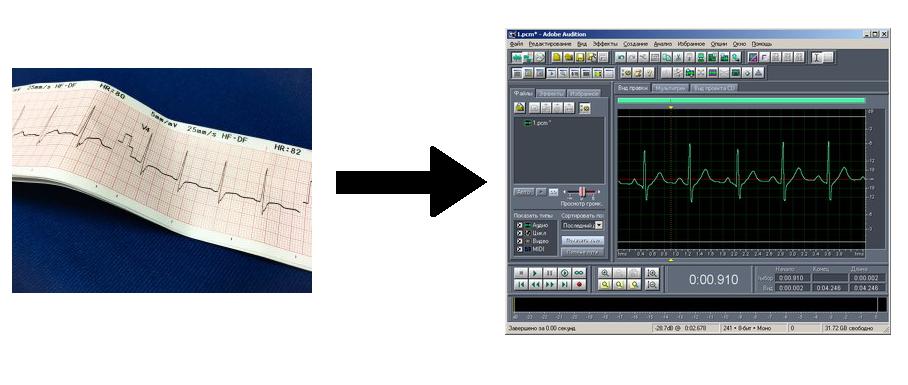
Many have repeatedly had to deal with the examination of the heart in medical institutions using a cardiograph. This unit measures the bioelectric activity of the heart by recording the result on a paper tape. Modern cardiographs record the measurement result not on paper, but in digital memory. However, paper tape is often used as the final carrier of recorded information. Visually, it is a long millimeter paper of small width, which is twisted into a roll. On paper, in addition to the millimeter grid, a certain graph is drawn full-length, which reflects the law of change of the measured value in time. The measured quantity, as I understand it, is the potential difference between the leads. Most often, several diagrams are represented on one tape at once, since potential differences between multiple leads are recorded. However, without going into details of medicine, in the future we will consider one of the first main graphs. In addition to the graphs, there is additional textual information on the tape: horizontal scale (mm / s), vertical (mm / mV), measured heart rate (beats / min) and so on.

The idea arose to convert this graphic into audio format, reproduce the result and listen to how it will sound.

According to preliminary analysis, we can conclude that the frequency composition of such a wave is not very saturated. In fact, these are low frequencies, including infrasound, which is not supposed to be heard. However, it will be possible to see how the woofer diffuser will repeat the vibrations, similar to the "vibrations" of the heart. In fact, due to the presence of capacitive differentiating circuits in the path of the signal from the PC sound card to the LF amplifier, the oscillations of the dynamic head will not exactly repeat the oscillations shown on the cardiogram. And this is on condition that no filters are installed anywhere that cut ultra-low frequencies. In addition, nonlinear distortions will be present, accompanied by multiple high-frequency harmonics. However, without taking into account the above analysis, we set the task as follows: convert the graph on paper to WAV format, so that when opening this file in the audio editor, the wave view coincides with the paper version and, moreover, the time scale corresponds.

First you need to estimate the quantization depth (vertical audio resolution of digital audio). I consider one of the standard: 8 or 16 bits. The second variant (16 bits) is 65536 samples vertically, which will correspond to 65536 pixels of a picture, which is a scan or photo of a cardiogram. This is a lot, and there is no point in it. If you take 8 bits - this is 256 samples, or 256 pixels of a picture. Now this is a more suitable option. In this case, the dynamic range of audio will be 6 * 8 = 48 dB. I do not know what the dynamic range of the cardiogram, but I think that no more. In the apparatus itself, it is naturally more, but the error is inevitable when the cardiogram is put on paper, especially when it comes to direct pen drawing. By the way, about the latter. I will not take into account the old patterns, which are drawn by a “radial” pen. Millimeter paper tape for such cardiograms is specific: vertical arcs of circles are applied instead of straight lines. As for the horizontal scale - the sampling rate - will be calculated based on the scale of the ECG and image size. The speed of reproduction will depend on this parameter, and it should correspond to the real “cardiogram speed”.
')
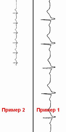
Cardiogram paper should be scanned in b / w with shades of gray in sufficient resolution. Then you need to resize the image so that the desired cardiogram fits into a 256 pixel wide strip. I found on the Internet a lot of images with cardiograms. As an example, consider two of them.



The first image, one can say, is almost ready. The image height is 431. Width is 1023. A wave in width completely fills the entire drawing. But the height must be left 256, cutting off the image above and below so that the wave is located approximately in the center.



The second image shows several cardiograms at once. Take the very first. After cropping, a 508 by 61 picture was obtained.



Without stretching the image vertically, we will make a picture at a height of 256, filling the created area with a white void. The wave should also be located approximately in the center. When cutting, I chose width 508 so as to leave as many as possible whole millimeter cells, which are also visible in the image.

Both images need to be converted to a view in which only a black graph is visible on a white background and nothing else. This is done elementary. Due to the fact that the graph is drawn much fatter than the millimeter grid, the desired result can be achieved in the graphical editor with the help of “brightness, contrast, saturation” adjustments. If the ideal transformation does not work, the excess “garbage” over the chart should be erased with the eraser tool. All images must be saved in monochrome BMP format. Thus, in the picture, only white and black colors will definitely remain.

Before proceeding to the description of the algorithm for converting images to WAV, it is worthwhile to stipulate some nuances that will simplify programming. The resulting images must be rotated 90 degrees counterclockwise (the width and height of the image will swap places). This is necessary in order to orient the beginning of the cardiogram with the beginning of the BMP file. It is known that the color data of each pixel of a BMP file is written to the file in order, line by line, starting from the bottom left corner. Then you need to open the pictures in the MS Paint editor (I have Windows XP) and save to 8-bit BMP (256 colors). Of course, there will be a "redefinition of information", but in this format, each pixel of the image corresponds to one byte, which is very convenient when programming. Byte "0" is a black pixel, and byte "255" is white. As a result, you should get something like the following (here two pictures are connected and halved).



As for the output format, we will not output to the standard WAV file, but to the RAW data (PCM) file. It also simplifies programming, because when outputting to WAV, you still need to take care of the 44-byte header. In the popular audio editor "Adobe Audition 1.5" PCM file opens without problems. Moreover, you can even output decimal PCM data to a text file in a column, having previously formed a specific text header. Oddly enough, Adobe Audition also opens such files.

We describe the conversion algorithm. And the algorithm is very simple: you need to analyze each line of the BMP file from the bottom up. The analysis will consist in counting white pixels in a row from left to right until black is encountered. The resulting non-negative integer values ​​must be written to the output PCM file in binary form. The size of the output file will be exactly the same as the height of the processed image. The quantization depth of 8 bits of PCM audio data format implies encoding of samples according to the same principle. The value “0” is the maximum negative value of the audio sample, the value “255” is the maximum positive, and “128” is the zero value (in the middle). For example, the PCM audio data file of silence will contain the same byte value "128". It is necessary to stipulate that in the line there may be several consecutive black pixels, depending on the thickness of the line of the cardiogram. But the described algorithm "catches" the upper envelope, which is quite enough. Moreover, the sharp peaks of the cardiogram, directed upwards, will be better grasped in this way.

Now you can start writing the text of the program. The program written in C is very simple and does not need detailed comments.

#include <stdio.h> // ,  ; int main(){ //  ; FILE *in,*out; //   ; unsigned long int h,i; //    ; unsigned char px,s; //     ; in=fopen("1.bmp","rb"); //   ; out=fopen("1.pcm","wb"); //   ; fseek(in,22,SEEK_SET); //    ,     fread(&h,4,1,in); //   (4 ); for(i=0;i<h;i++){ // -   ; fseek(in,0x436+i*256,SEEK_SET); //   i-  s=0; //  ( ); do{ //  ; fread(&px,1,1,in); //  ; s+=1; //   ; }while(px); // ,     ; fwrite(&s,1,1,out); //     ; } fclose(in); //  ; fclose(out); //  ; return 0; //  ; } 

After the program is executed on the file "1.bmp" a file "1.pcm" will be created in the same directory with the program. When you try to open a file in Adobe Audition, the following window should pop up.



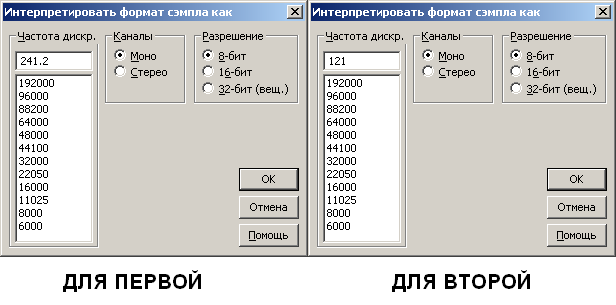
It is necessary to select “Mono”, “8-bit” and type the sampling rate in the input field based on the calculation: f = h / (s / v), where h is the height of the image (it is also the number of samples in the audio), s - cardiogram length in millimeters, v - cardiogram scale in mm / sec. The last parameter is written on the cardiogram. On the first cardiogram nothing is written, but the scale, as a rule, is often 25 mm / sec. Calculations of sample rates in Excel for our examples are shown in the figure below.



As mentioned above, we enter in the appropriate field the necessary sampling rates for each of the examples. You can even enter decimals, anyway, then there will be an automatic rounding to the whole.



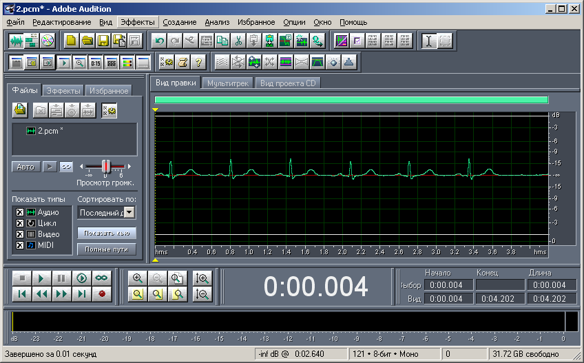
When you click “OK”, we agree that we work with “Unsigned 8 bit” samples (there will be another window), after which the waveform of our file will unfold in the main field of the sound editor. Note that this view will be presented “upside down”, and for full compliance with the paper version, you should invert the wave in the corresponding menu. As a result, it will look like this.



The second cardiogram looks "quieter", as it was initially not very large in size.



Unfortunately, not all sound cards allow you to play audio at an arbitrary sampling rate, more precisely, the vast majority are not able to. In order to correctly play the file, you must perform the function "Convert a sample type." We will convert to the nearest standard value of 8000 Hz, at the same time we will increase the resolution in amplitude to 16 bits. The latter is necessary for accuracy at the interpolation stage when upsampling. If you leave 8 bits, the remaining spectrum will be filled with quantization noise. Incidentally, this procedure could be performed programmatically at the BMP-PCM conversion stage, even using interpolation. But one of the goals was the simplicity of the program code.

After the upsampling operation, you can listen and enjoy the result. You can save the result in a standard wav or mp3 file. It sounds exactly the same as I expected initially.

Using this link you can download the rar-archive, which contains two wave files with the result.