Numerical methods for solving elliptic equations
Introduction
The most common elliptic equation is the Poisson equation.
Many problems of mathematical physics, such as the problem of stationary temperature distribution in a solid, diffusion problems, the distribution of an electrostatic field in a nonconducting medium in the presence of electric charges, and many others, are reduced to solving this equation.
In the case of several measurements, numerical methods are used to solve elliptic equations, which allow transforming differential equations or their systems into systems of algebraic equations. The accuracy of the solution is determined by the grid step, the number of iterations and the computer's bit grid [1]
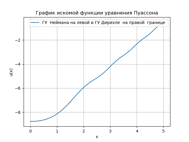
The purpose of the publication is to obtain a solution to the Poisson equation for the Dirichlet and Neumann boundary conditions, to investigate the convergence of the relaxation method of the solution with examples.
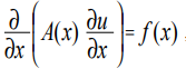
The Poisson equation refers to equations of elliptic type and in the one-dimensional case has the form [1]:
')
 (one)
(one)where x is the coordinate; u (x) is the desired function; A (x), f (x) are some continuous coordinate functions.
We solve the one-dimensional Poisson equation for the case A = 1, which in this case takes the form:
 (2)
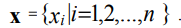
(2)Let us set a uniform coordinate grid with step ∆ on the segment [xmin, xmax]:
 (3)
(3)The boundary conditions of the first kind (Dirichlet conditions) for the problem in question can be represented as:
 (four)
where x1, xn are the coordinates of the boundary points of the region [xmin, xmax]; g1, g2 - some
constants.
The boundary conditions of the second kind (Neumann conditions) for the problem in question can be represented as:
 (five)
Conducting the discretization of the Dirichlet boundary conditions on a uniform coordinate grid (3) using the finite difference method, we obtain:
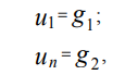 (6)
(6)where u1, un are the values of the function u (x) at the points x1, xn, respectively.
Conducting a discretization of the Neumann boundary conditions on the grid (3), we obtain:
 (7)
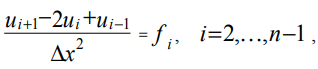
(7)Carrying out the discretization of equation (2) for the internal points of the grid, we obtain:
 (eight)
where ui, fi are the values of the functions u (x), f (x) at the grid point with the coordinate xi.
Thus, as a result of discretization, we obtain a system of linear algebraic equations of dimension n containing n - 2 equations of the form (8) for the interior points of the domain and equations (6) and (7) for two boundary points [1].
Below is a Python listing of the numerical solution of equation (2) with boundary conditions (4) - (5) on a grid (3).
Solution listing
from numpy import* from numpy.linalg import solve import matplotlib.pyplot as plt x0=0# xn=5# n=100# dx=(xn-x0)/(n-1)# dx x=[i*dx+x0 for i in arange(0,n,1)]# dx def f(i):# return 2*sin(x[i]**2)+cos(x[i]**2) v1=1.0# (1 - , 2 - ) g1=0.0# v2=2.0#' (1 - , 2 - ) g2=-0.5# a=zeros([n,n])# nxn b=zeros([1,n])# - 1 xn # , # # v1, v2 b[0,n-1]=g1; if v1==1: a[0,0]=1 elif v1==2: a[0,0]=-1/dx a[0,1]=1/dx; else: print(' v1 ') b[0,n-1]=g2; if v2==1: a[n-1,n-1]=1 elif v2==2: a[n-1,n-1]=1/dx a[n-1,n-2]=-1/dx; else: print(' v2 ') # , # for i in arange(1, n-1,1): a[i,i]=-2/dx**2 a[i,i+1]=1/dx**2 a[i,i-1]=1/dx**2 b[0,i]=f(i) u=linalg.solve(a,bT).T# def viz(v1,v2): if v1==v2==1: return " " elif v1==1 and v2==2: return " " elif v2==1 and v2==1: return " " plt.figure() plt.title(" ") y=[f(i) for i in arange(0,n,1)] plt.plot(x,y) plt.grid(True) plt.xlabel('x') plt.ylabel('f(x)') plt.figure() plt.title(" ") plt.xlabel('x') plt.ylabel('u(x)') plt.plot(x,u[0,:],label='%s'%viz(v1,v2)) plt.legend(loc='best') plt.grid(True) plt.show() We get:


The program I developed in Python is convenient for analyzing boundary conditions. The reduced Python solution algorithm uses the Numpy function - u = linalg.solve (a, bT) .T to solve a system of algebraic equations, which improves the speed with a square matrix {a}. However, with an increase in the number of measurements, it is necessary to switch to the use of a three diagonal matrix, a solution for which becomes even more complicated for a very simple task. I found an example on the forum:
An example of a solution with a three-diagonal matrix
from __future__ import print_function from __future__ import division import numpy as np import time ti = time.clock() m = 1000 A = np.zeros((m, m)) B = np.zeros((m, 1)) A[0, 0] = 1 A[0, 1] = 2 B[0, 0] = 1 for i in range(1, m-1): A[i, i-1] = 7 A[i, i] = 8 A[i, i+1] = 9 B[i, 0] = 2 A[m-1, m-2] = 3 A[m-1, m-1] = 4 B[m-1, 0] = 3 print('A \n', A) print('B \n', B) x = np.linalg.solve(A, B) # solve A*x = B for x print('x \n', x) print('NUMPY time', time.clock()-ti, 'seconds') The program of numerical solution on the Dirichlet problem uniform for each direction of the grid for the convection-diffusion equation
[2] (9)
(9)We use approximations by central differences for the convective term and an iterative relaxation method. For the dependence of the rate of convergence on the relaxation parameter for the numerical solution of the problem with / (x) = 1 and 6 (x) = 0.10. In the grid problem:
 (ten)
(ten)Imagine the matrix A as a sum of diagonal, lower triangular and upper triangular matrices:
 (ten)
(ten)The relaxation method corresponds to the use of the iterative method :
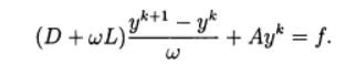 (eleven)
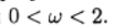
With
 \ talk about upper relaxation, when
  - about lower relaxation.
Program Listing
from numpy import * """ - . .""" def relaxation(b, f, I1, I2, n1, n2, omega, tol = 1.e-8): h1 = I1 / n1 h2 = I2 / n2 d = 2. / h1**2 + 2. / h2**2 y = zeros([n1+1, n2+1]) ff = zeros([n1+1, n2+1]) bb = zeros([n1+1, n2+1]) for j in arange(1,n2,1): for i in arange(1,n1,1): ff [i,j] = f(i*h1, j*h2) bb[i,j] = b(i*h1, j*h2) # - 10000 for k in arange(1, 10001,1): rn = 0. for j in arange(1,n2,1): for i in arange(1,n1,1): rr = - (y[i-1,j] - 2.*y [i, j] + y[i+1,j]) / h1**2 \ - (y[i,j-1] - 2.*y [i,j] + y[i,j+1]) / h2**2 \ + bb[i,j]*(y [i+1,j] - y [i-1,j]) / (2.*h1) - ff [i,j] rn = rn + rr**2 y[i,j] = y[i,j] - omega * rr / d rn = rn*h1*h2 if rn < tol**2: return y, k print (' :') print (' 10000 =',sqrt(rn)) import matplotlib.pyplot as plt bcList = [0., 10.] sglist = ['-','--'] kk = 0 for bc in bcList: I1 = 1. I2 = 1. def f(x,y): return 1. def b(x,y): return bc n1 = 25 n2 = 25 m = 20 om = linspace(1., 1.95, m) it = zeros(([m])) for k in arange(0,m,1): omega = om[k] y, iter = relaxation(b, f, I1, I2, n1, n2, omega, tol=1.e-6) it[k] = iter s1= 'b =' + str(bc) sg = sglist[kk] kk = kk+1 plt.plot( om,it, sg, label = s1) plt.title(" \n \n $\\omega$") plt.xlabel('$\\omega$') plt.ylabel('iterations') plt.legend(loc=0) plt.grid(True) plt.show( )We get:
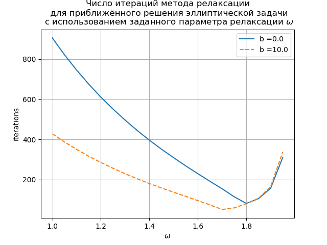
The graph shows the dependence of the number of iterations on the relaxation parameter for the Poisson equation (b (x) = 0) and the convection-diffusion equation (b (x) = 10). For the grid Poisson equation, the optimal value of the relaxation parameter is found analytically, and the iterative method converges at
 .
.Findings:
- The solution of an elliptic problem in Python with a flexible system for setting boundary conditions is given.
- It is shown that the relaxation method has an optimal range ( a) relaxation parameter.
References:
- Ryndin E.A. Methods for solving problems of mathematical physics. - Taganrog:
Publishing house TSURE, 2003. - 120 p. - PN Vabishchevich. Numerical methods: Computational practical work. - M .: Book House
LIBROCOM, 2010. - 320 p.
Source: https://habr.com/ru/post/418981/
All Articles