The best reports about machine learning with ICML 2018 according to the version of Yandex employees
From July 10 to July 15, the ICML conference, one of the world's largest in machine learning, was held in Stockholm. This year, it was visited by a record number of participants - 7,000. Among them were Yandex employees who represented CatBoost and DeepHD technologies, Toloka, Zen and Translator services, unmanned vehicles and other products. Today they will share with Habr's readers a collection of reports that they remember most.
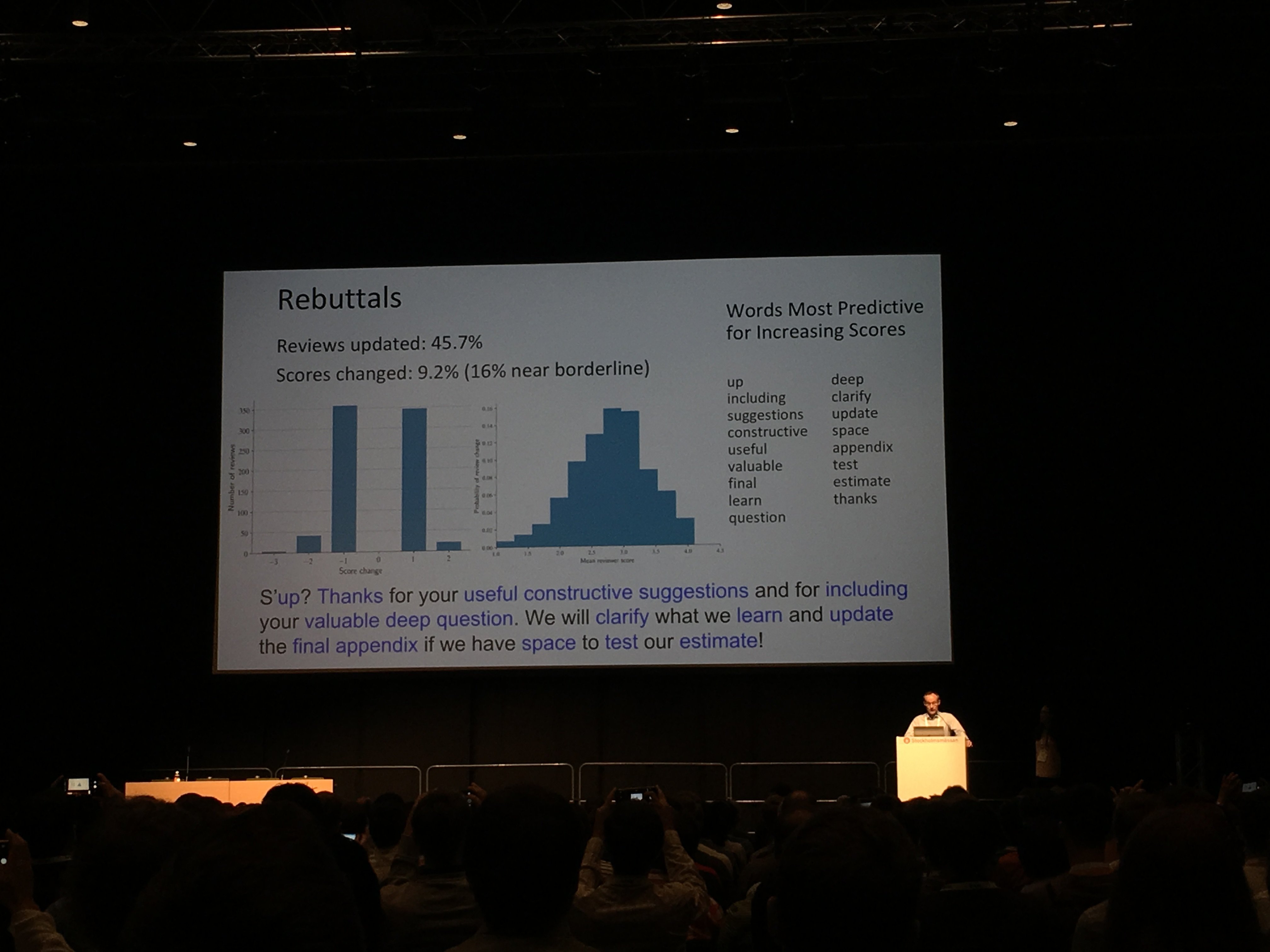
By the way, in the photo above, the organizers' joke are statistics on the words from the letters of those who sent their report to the conference. More precisely, from letters with answers to criticism of reviewers, which led to the reception of the report. Here is the "perfect" answer, from the point of view of machine learning. But we digress, go to the review of the five best reports (all the headlines are clickable and lead to the work of the speakers).
One of the most interesting reports about generative models and training presentations at the conference.
')
Prehistory
Variational autocoders (VAE) try to model the distribution of observable data following process:
1. First, from some a priori distribution choose "hidden" variable .
2. Then using neural network decoder with parameters distribution parameters are obtained from it .
3. From the distribution obtained choose the next object.
Such a formulation allows building very complex models and well-interpreted representations from simple bricks. For example, if Is a two-dimensional normal distribution, and - 724-dimensional Bernoulli vector, VAE successfully learns the variety of MNIST numbers.
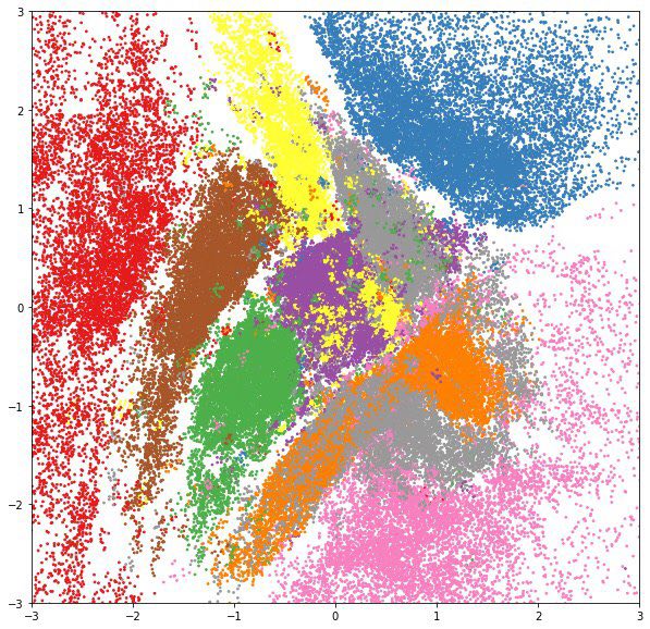
If in the resulting space in place of points draw the expectation of the corresponding distributions , we will see that the model carefully laid the variety of numbers on the plane.

And if for each class of numbers from the test set to draw a posteriori distribution in a separate color, we will see that the hidden variables learn very useful ideas: on such two-dimensional features it is much easier to teach the classifier, and it definitely does not need a lot of marked up data.
Likelihood of observable data in this model is written in the form:
If a given by a deep neural network, we have no chance of taking this integral analytically, so direct maximization of likelihood is impossible. Instead, use the so-called variational Bayesian output:
- For each object of the training sample, an auxiliary distribution is introduced described by parameter . Task - as closely as possible approximate the posterior distribution . In other words, it predicts from which observable object was obtained .
- The lower estimate of the likelihood logarithm of the sample is recorded:
This lower score is also called ELBO (Evidence Lower Bound) - the lower limit of reasonableness. It is exactly equal to the log likelihood if .
- The resulting score is maximized by and a stochastic gradient descent, and the stochastic gradient of the internal integral is obtained either by reparametrization trick , or by using a log-derivative trick (also known as score function estimator, also known as REINFORCE).
Because to store and optimize parameters for each sample object is too expensive, an additional neural network-encoder is introduced, which accepts input and returns . This approach is called a depreciated variational output. It was the use of amortized output that allowed us to study complex hierarchical probabilistic models on big data.
Too smart decoder
When we limit simple family of distributions (for example, normal distributions with diagonal covariance matrices), learns useful data views. Simple arithmetic in space You can change the hairstyle of a person in a photo or mix tunes.

However, simple models in which all elements of the vector independent provided , do not do very well with complex data, such as texts or high-resolution images. It is reasonable to try to use as complex “neural network” distributions: autoregressive networks, such as WaveNet or PixelCNN, normalizing flows, for example, RealNVP, nested VAE, or even -GAN.
When trying to train VAE with such decoders, researchers face great difficulties: the “too smart” decoder itself “eats” all the entropy in the data and stops looking at the hidden variable at all. and turn out to be independent, and it’s impossible to get useful views from a hidden variable. Different articles have suggested ways to get around this problem, but basically they boil down to either simplifying the decoder or different hacks when learning. The authors of this article offer a first fundamental explanation of the causes of this effect and ways to combat it.
The main ideas of the article
- Apparatus from Information Bottleneck Theory is applied to the task of learning views. The authors propose to consider mutual information between and . When mutual information is equal , hidden variable compresses lossless data: we get the perfect auto-coding. When the mutual information is equal to zero, the hidden variable is independent of the data, the decoder “devoured” all the entropy. In order to train useful ideas, we want to get a variant in the middle: the hidden variable should describe important information about the object (for example, the shape of the face, the color of the eyes, ...) and throw away the details (the colors of specific pixels, textures).
- It is proposed to look at VAE from an alternative position: now let the main part of the model , but and - approximation for and marginal distribution .
- For fixed considered lower and upper estimates for mutual information, depending on and :
Where - data entropy - loss in compression and - KL divergence between and

Each family of models corresponds to a convex set of points in the RD space, the shape of this set depends on the “balance of forces” between the encoder and the decoder.
- It is shown that optimization of ELBO is equivalent to minimization , i.e. searching for a point with a tangent coefficient on the boundary of the set. If the decoder is flexible enough unable to approximate well , it is not profitable for models to put additional information into a latent variable: from the ELBO point of view, it is cheaper to learn it with a decoder.
- To build the most useful ideas, the authors propose to optimize where - a hyperparameter responsible for the balance between the encoder and the decoder.
- The authors experimentally showed that by varying , it is possible to learn representations with different levels of abstraction: from autoencoder ( ), which compresses lossless data, to “auto decoder” ( ), which completely ignores the data. Picking up the value , you can get a "semantic encoder", which encodes only the general form of the object, or "syntactic encoder", which is able to recover small details. In this case, all experiments were carried out with a superpowerful autoregressive PixelCNN ++ decoder, which until then had not been able to use in VAE.

The authors set themselves the task of displaying music (as a sequence of characters) in an adequate hidden space while preserving the semantics. This will allow to solve the problem of continuing the musical sequence and automatically creating smooth "transitions" between different fragments. It is proposed to use VAE.
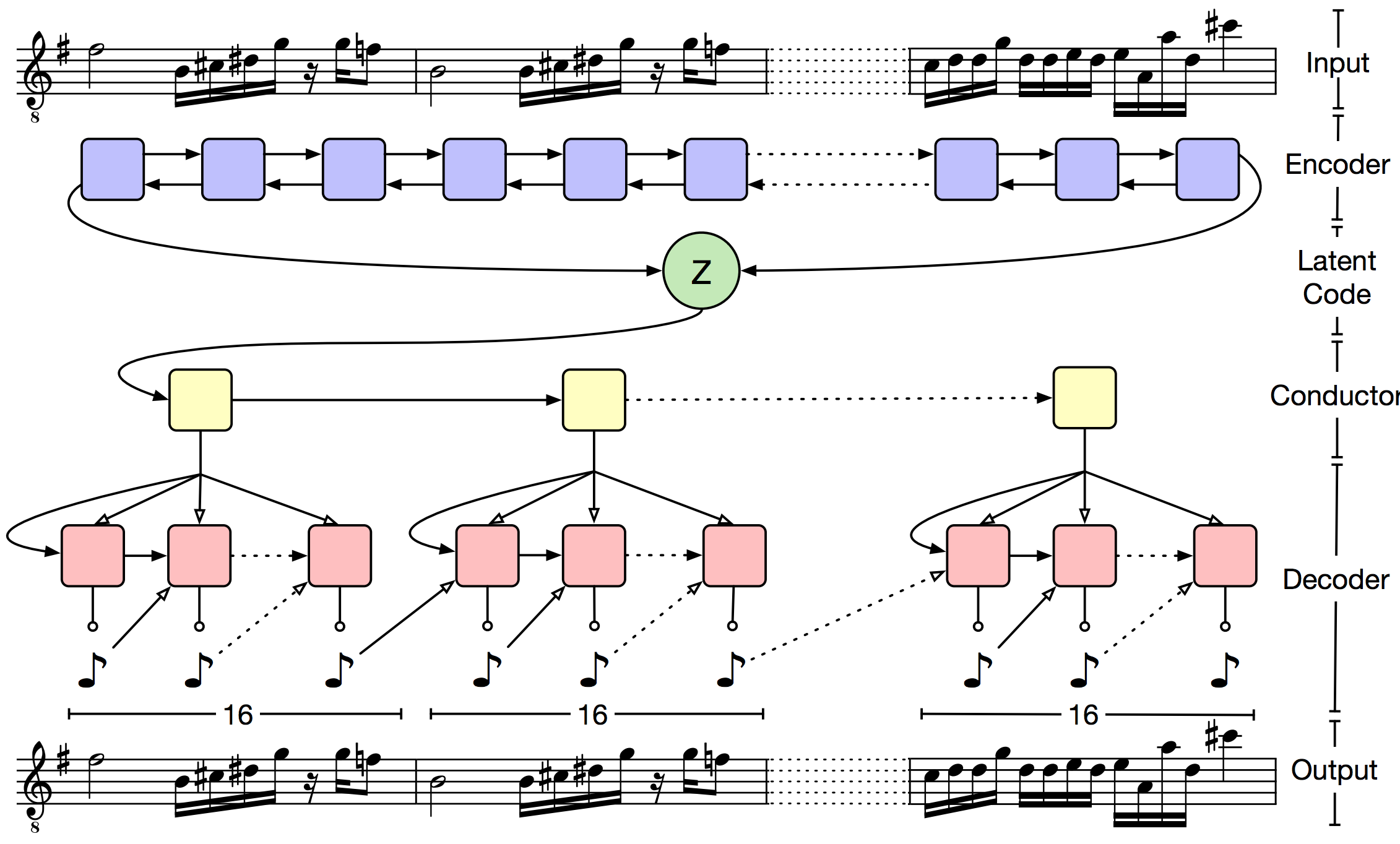
The main problem of VAE is that the decoder very quickly forgets the “hidden” code. The authors propose to deal with this through a hierarchical decoder. The output sequence is divided into small pieces (in the article, the music was broken into bars). The "hidden" code is fed to the input of the upper-level decoder, which returns the embedding for the beat. And then the low-level LSTM predicts the notes inside the beat. Formally, this approach does not solve the problem of forgetting, but in practice it turns out that the resulting sequences correspond much better to the original piece.
The encoder is a bidirectional LSTM. Hidden layers and concatenated and used to predict distribution parameters :
The overall network layout looks like this:
For quality assessment, Lakh MIDI Dataset is used, which contains about one and a half million midi files. The authors used only tracks with a size of 4/4. On short sequences (prediction of the next two bars), the quality of MusicVAE is comparable to the classic VAE. However, already on the prediction of 16 cycles, the error rate of the classic VAE is more than 27%, and for the hierarchical method in the range of 5-11%. It is also shown that the hierarchical method gives a smoother interpolation between fragments of music.
For a snack: over the latent code vectors you can make arithmetic operations. For example, the authors built vectors for 5 musical characteristics (C diatonic membership, note density, average interval, 16th and 8th note syncopation). With some weights, the vector of characteristics can be added to the sampled vectors, and the resulting sequence obtained at the output of the decoder will more or less correspond to a given characteristic depending on the weight.
When training VAE, it is important to choose the right form. , since the accuracy of the lower likelihood estimate depends on its expressiveness. A good family should satisfy the following properties:
- It is quite flexible (ideally, it can approximate any distribution).
- From it you can quickly get a sample.
- The resulting sample is easy to calculate the credibility.
- The complexity of these operations grows linearly with increasing dimension.
One of the approaches to the construction of such families is normalizing flows. They are based on the variable change formula: if a random variable transform with a reversible differentiable function the density of magnitude equals where - Jacobian functions . By choosing a family of functions in which the Jacobian determinant can be effectively considered, it is possible to obtain complex distributions, transforming Gaussian noise.

In the previous approach ( Inverse Autoregressive Flow ) each element of the vector undergoes affine transformation, the parameters of which are set by an autoregressive neural network (for example, MADE or PixelCNN), looking at previous elements , .
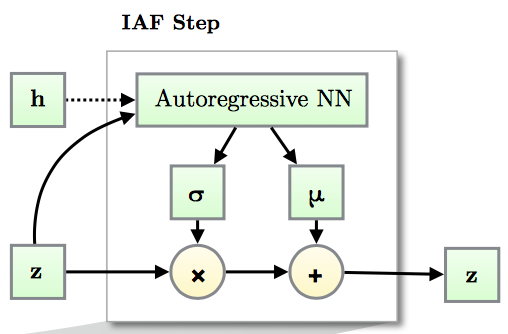
Due to the autoregressive network structure, the Jacobian of the resulting transformation is lower triangular, which means that its determinant can be easily calculated as the product of diagonal elements.
IAF is a powerful family, but due to the fact that an affine transformation is used at each step, it is not able to approximate well multimodal distributions.
The main ideas of the authors of the article
- Instead of affine transformation in IAF, use a miniature neural network with positive weights and strictly monotonous activations.
- The resulting normalizing flow is a universal approximator for distributions.
- Two architectures of transforming networks were proposed and a mechanism for scaling to large dimensions was described using conditional batch normalization.
- Experiments show that NAF can really learn multimodal things.

If one phrase - this is super-resolution without GAN'ov.
The classic approach to the super-resolution task (obtaining a clean image from a more noisy one) is to input noisy images to the algorithm and teach them to predict a clean image. But what if we don't have clean images? This is true for processing photos from telescopes, MRI images and other similar tasks. The idea proposed in the article is to teach the network on noisy images. But it is necessary that the noise in the images was on average zero. The authors conclude: "... we can find out about the network learners". In the datasets they consider, the results are not much worse, and sometimes even better than the state of the art. In addition, the speed and speed of learning is much higher.
The authors tried to work with frames from the video, however, they didn’t really make a super-resolution video yet - the recovered image “jumps”.
Despite the fact that ICML is devoted to machine learning, there are many good reports on related areas. So, in the section devoted to the work with distributed computations, an interesting algorithmic report on graphs was presented.
Suppose we want to solve some problem on the graph. The task is abstract enough to describe it in terms of formal logic. For example, we are given a graph of user communications, and we want to detect anomalies in it (bot networks, fraud) or to identify links with communities of people.
For these and many other tasks in teaching models related to graphs, the selection of entities called k-core is well suited.
It is important to note that it is not only the approach to extracting these k-core that is of interest, but also the ability to do it efficiently, in a distributed way, and, if possible, also on a stream. These are the implementations that were immediately presented in this report.
Definitions
Let be - undirected graph with tops and ribs - subgraph . For each vertex we denote by the degree of this vertex, and for denote as - degree in the subgraph .
-Core - maximum subgraph such that for we have in other words - the degree of any vertex does not exceed . Also called such a graph - degenerate.
It is said that the top has coreness number if she belongs -core but not owned -core.
Core labeling graph - a graph where each vertex is labeled with its coreness number. It is worth noting that core labeling is unique and defines a hierarchical decomposition. .
Approximate -core - subgraph at such that $ inline $ ∀v ∈ H dH (v) ≥ (1 - ε) k $ inline $ .
In the figure below, examples 3 − core and -approximate 3-core.
The idea of the algorithm
The basic idea is to more confidently throw out the ribs in dense areas and less confidently in sparse ones.
Brief description of the algorithm:
- we throw out edges from the graph with probability ;
- for each vertex we define its coreness number, that is, we do core labeling, we find the maximum -core, and add all its vertices to the set ;
- delete from all edges, both ends of which are in ;
- doing the same thing, increasing twice as long as possible.
Pseudocode:

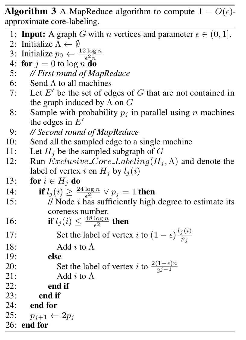
Let us analyze how this algorithm can be implemented in the MapReduce ideology for parallel computing.
It is argued that when starting probability the algorithm is executed no more iterations. In the first iteration, by throwing out the edges, we get some subgraph . At the second iteration on each machine we do core labeling . Save the vertices with the largest core number in some set . At the third iteration, we send a set to all the machines. and in parallel we throw out edges, both ends of which are in get . Further, with probability doing the same time.
Pseudocode:
Note
Let's return to the search for communities on the graph. Consider a graph of social connections. For example, a graph where vertices correspond to user pages on a social network, and edges indicate that users have added each other as friends. We also know about some subset of pages information about where this user is studying (city, university, faculty, specialty, group).
In this case, the hierarchy with -core can be interpreted as follows: kernels of a higher order reflect the group in which the student is studying - the community is rather narrow, but with a high density of connections in it. The core of the order below will reflect the community-specialty of this user - the links are generally smaller, but they are fairly dense. Moving further along the hierarchy we find the community and the faculty, and the university.
The exploitation of this idea for spam analysts looks less obvious, but is similar in essence. If we have an idea about which kernels are considered good, then using factors like “maximum order -core to which the user belongs, density -core user ", as well as the ratio of the nearest entities may well help in the detection of suspicious nodes and the identification of botnet patterns.
Today we talked about only five reports, but there were more of them at the ICML conference. If specialists in the field of machine learning would be interested in such a format, then we could repeat it in the future.
By the way, in the photo above, the organizers' joke are statistics on the words from the letters of those who sent their report to the conference. More precisely, from letters with answers to criticism of reviewers, which led to the reception of the report. Here is the "perfect" answer, from the point of view of machine learning. But we digress, go to the review of the five best reports (all the headlines are clickable and lead to the work of the speakers).
1. Fixing the broken ELBO
One of the most interesting reports about generative models and training presentations at the conference.
')
Prehistory
Variational autocoders (VAE) try to model the distribution of observable data following process:
1. First, from some a priori distribution choose "hidden" variable .
2. Then using neural network decoder with parameters distribution parameters are obtained from it .
3. From the distribution obtained choose the next object.
Such a formulation allows building very complex models and well-interpreted representations from simple bricks. For example, if Is a two-dimensional normal distribution, and - 724-dimensional Bernoulli vector, VAE successfully learns the variety of MNIST numbers.
If in the resulting space in place of points draw the expectation of the corresponding distributions , we will see that the model carefully laid the variety of numbers on the plane.
And if for each class of numbers from the test set to draw a posteriori distribution in a separate color, we will see that the hidden variables learn very useful ideas: on such two-dimensional features it is much easier to teach the classifier, and it definitely does not need a lot of marked up data.
Likelihood of observable data in this model is written in the form:
If a given by a deep neural network, we have no chance of taking this integral analytically, so direct maximization of likelihood is impossible. Instead, use the so-called variational Bayesian output:
- For each object of the training sample, an auxiliary distribution is introduced described by parameter . Task - as closely as possible approximate the posterior distribution . In other words, it predicts from which observable object was obtained .
- The lower estimate of the likelihood logarithm of the sample is recorded:
This lower score is also called ELBO (Evidence Lower Bound) - the lower limit of reasonableness. It is exactly equal to the log likelihood if .
- The resulting score is maximized by and a stochastic gradient descent, and the stochastic gradient of the internal integral is obtained either by reparametrization trick , or by using a log-derivative trick (also known as score function estimator, also known as REINFORCE).
Because to store and optimize parameters for each sample object is too expensive, an additional neural network-encoder is introduced, which accepts input and returns . This approach is called a depreciated variational output. It was the use of amortized output that allowed us to study complex hierarchical probabilistic models on big data.
Too smart decoder
When we limit simple family of distributions (for example, normal distributions with diagonal covariance matrices), learns useful data views. Simple arithmetic in space You can change the hairstyle of a person in a photo or mix tunes.
However, simple models in which all elements of the vector independent provided , do not do very well with complex data, such as texts or high-resolution images. It is reasonable to try to use as complex “neural network” distributions: autoregressive networks, such as WaveNet or PixelCNN, normalizing flows, for example, RealNVP, nested VAE, or even -GAN.
When trying to train VAE with such decoders, researchers face great difficulties: the “too smart” decoder itself “eats” all the entropy in the data and stops looking at the hidden variable at all. and turn out to be independent, and it’s impossible to get useful views from a hidden variable. Different articles have suggested ways to get around this problem, but basically they boil down to either simplifying the decoder or different hacks when learning. The authors of this article offer a first fundamental explanation of the causes of this effect and ways to combat it.
The main ideas of the article
- Apparatus from Information Bottleneck Theory is applied to the task of learning views. The authors propose to consider mutual information between and . When mutual information is equal , hidden variable compresses lossless data: we get the perfect auto-coding. When the mutual information is equal to zero, the hidden variable is independent of the data, the decoder “devoured” all the entropy. In order to train useful ideas, we want to get a variant in the middle: the hidden variable should describe important information about the object (for example, the shape of the face, the color of the eyes, ...) and throw away the details (the colors of specific pixels, textures).
- It is proposed to look at VAE from an alternative position: now let the main part of the model , but and - approximation for and marginal distribution .
- For fixed considered lower and upper estimates for mutual information, depending on and :
Where - data entropy - loss in compression and - KL divergence between and
Each family of models corresponds to a convex set of points in the RD space, the shape of this set depends on the “balance of forces” between the encoder and the decoder.
- It is shown that optimization of ELBO is equivalent to minimization , i.e. searching for a point with a tangent coefficient on the boundary of the set. If the decoder is flexible enough unable to approximate well , it is not profitable for models to put additional information into a latent variable: from the ELBO point of view, it is cheaper to learn it with a decoder.
- To build the most useful ideas, the authors propose to optimize where - a hyperparameter responsible for the balance between the encoder and the decoder.
- The authors experimentally showed that by varying , it is possible to learn representations with different levels of abstraction: from autoencoder ( ), which compresses lossless data, to “auto decoder” ( ), which completely ignores the data. Picking up the value , you can get a "semantic encoder", which encodes only the general form of the object, or "syntactic encoder", which is able to recover small details. In this case, all experiments were carried out with a superpowerful autoregressive PixelCNN ++ decoder, which until then had not been able to use in VAE.
2. A Hierarchical Latent Vector Model for Learning Long-Term Structure in Music
The authors set themselves the task of displaying music (as a sequence of characters) in an adequate hidden space while preserving the semantics. This will allow to solve the problem of continuing the musical sequence and automatically creating smooth "transitions" between different fragments. It is proposed to use VAE.
The main problem of VAE is that the decoder very quickly forgets the “hidden” code. The authors propose to deal with this through a hierarchical decoder. The output sequence is divided into small pieces (in the article, the music was broken into bars). The "hidden" code is fed to the input of the upper-level decoder, which returns the embedding for the beat. And then the low-level LSTM predicts the notes inside the beat. Formally, this approach does not solve the problem of forgetting, but in practice it turns out that the resulting sequences correspond much better to the original piece.
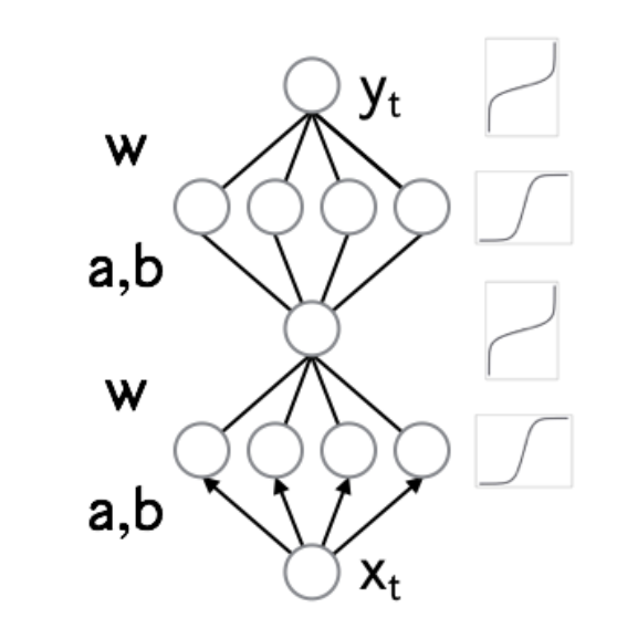
The encoder is a bidirectional LSTM. Hidden layers and concatenated and used to predict distribution parameters :
The overall network layout looks like this:
For quality assessment, Lakh MIDI Dataset is used, which contains about one and a half million midi files. The authors used only tracks with a size of 4/4. On short sequences (prediction of the next two bars), the quality of MusicVAE is comparable to the classic VAE. However, already on the prediction of 16 cycles, the error rate of the classic VAE is more than 27%, and for the hierarchical method in the range of 5-11%. It is also shown that the hierarchical method gives a smoother interpolation between fragments of music.
For a snack: over the latent code vectors you can make arithmetic operations. For example, the authors built vectors for 5 musical characteristics (C diatonic membership, note density, average interval, 16th and 8th note syncopation). With some weights, the vector of characteristics can be added to the sampled vectors, and the resulting sequence obtained at the output of the decoder will more or less correspond to a given characteristic depending on the weight.
3. Neural Autoregressive Flows
When training VAE, it is important to choose the right form. , since the accuracy of the lower likelihood estimate depends on its expressiveness. A good family should satisfy the following properties:
- It is quite flexible (ideally, it can approximate any distribution).
- From it you can quickly get a sample.
- The resulting sample is easy to calculate the credibility.
- The complexity of these operations grows linearly with increasing dimension.
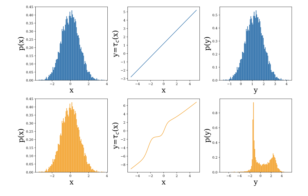
One of the approaches to the construction of such families is normalizing flows. They are based on the variable change formula: if a random variable transform with a reversible differentiable function the density of magnitude equals where - Jacobian functions . By choosing a family of functions in which the Jacobian determinant can be effectively considered, it is possible to obtain complex distributions, transforming Gaussian noise.
In the previous approach ( Inverse Autoregressive Flow ) each element of the vector undergoes affine transformation, the parameters of which are set by an autoregressive neural network (for example, MADE or PixelCNN), looking at previous elements , .
Due to the autoregressive network structure, the Jacobian of the resulting transformation is lower triangular, which means that its determinant can be easily calculated as the product of diagonal elements.
IAF is a powerful family, but due to the fact that an affine transformation is used at each step, it is not able to approximate well multimodal distributions.
The main ideas of the authors of the article
- Instead of affine transformation in IAF, use a miniature neural network with positive weights and strictly monotonous activations.
- The resulting normalizing flow is a universal approximator for distributions.
- Two architectures of transforming networks were proposed and a mechanism for scaling to large dimensions was described using conditional batch normalization.
- Experiments show that NAF can really learn multimodal things.
4. Noise2Noise: Learning Image Restoration without Clean Data
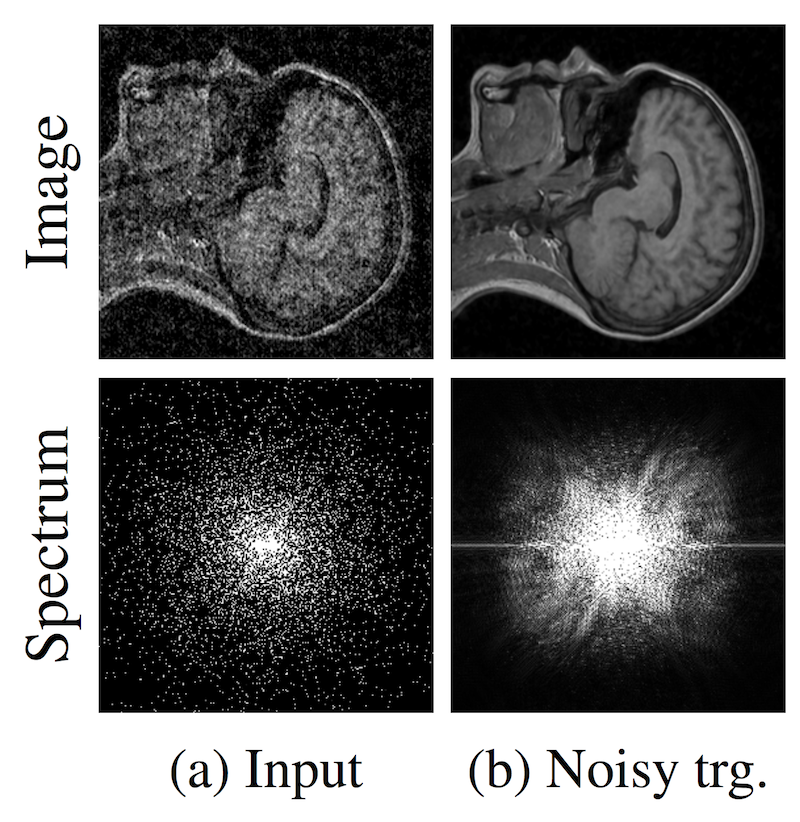
If one phrase - this is super-resolution without GAN'ov.
The classic approach to the super-resolution task (obtaining a clean image from a more noisy one) is to input noisy images to the algorithm and teach them to predict a clean image. But what if we don't have clean images? This is true for processing photos from telescopes, MRI images and other similar tasks. The idea proposed in the article is to teach the network on noisy images. But it is necessary that the noise in the images was on average zero. The authors conclude: "... we can find out about the network learners". In the datasets they consider, the results are not much worse, and sometimes even better than the state of the art. In addition, the speed and speed of learning is much higher.
The authors tried to work with frames from the video, however, they didn’t really make a super-resolution video yet - the recovered image “jumps”.
5. Approximate k-core graph decomposition
Despite the fact that ICML is devoted to machine learning, there are many good reports on related areas. So, in the section devoted to the work with distributed computations, an interesting algorithmic report on graphs was presented.
Suppose we want to solve some problem on the graph. The task is abstract enough to describe it in terms of formal logic. For example, we are given a graph of user communications, and we want to detect anomalies in it (bot networks, fraud) or to identify links with communities of people.
For these and many other tasks in teaching models related to graphs, the selection of entities called k-core is well suited.
It is important to note that it is not only the approach to extracting these k-core that is of interest, but also the ability to do it efficiently, in a distributed way, and, if possible, also on a stream. These are the implementations that were immediately presented in this report.
Definitions
Let be - undirected graph with tops and ribs - subgraph . For each vertex we denote by the degree of this vertex, and for denote as - degree in the subgraph .
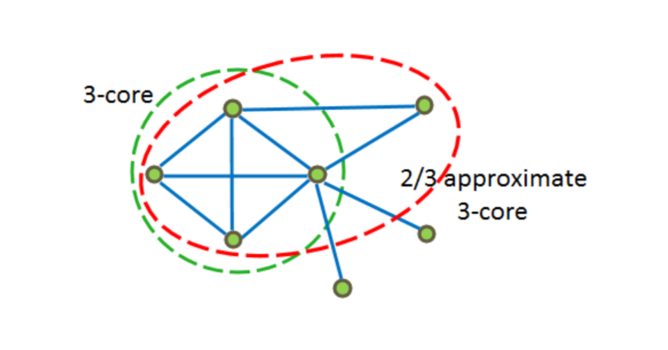
-Core - maximum subgraph such that for we have in other words - the degree of any vertex does not exceed . Also called such a graph - degenerate.
It is said that the top has coreness number if she belongs -core but not owned -core.
Core labeling graph - a graph where each vertex is labeled with its coreness number. It is worth noting that core labeling is unique and defines a hierarchical decomposition. .
Approximate -core - subgraph at such that $ inline $ ∀v ∈ H dH (v) ≥ (1 - ε) k $ inline $ .
In the figure below, examples 3 − core and -approximate 3-core.
The idea of the algorithm
The basic idea is to more confidently throw out the ribs in dense areas and less confidently in sparse ones.
Brief description of the algorithm:
- we throw out edges from the graph with probability ;
- for each vertex we define its coreness number, that is, we do core labeling, we find the maximum -core, and add all its vertices to the set ;
- delete from all edges, both ends of which are in ;
- doing the same thing, increasing twice as long as possible.
Pseudocode:
Let us analyze how this algorithm can be implemented in the MapReduce ideology for parallel computing.
It is argued that when starting probability the algorithm is executed no more iterations. In the first iteration, by throwing out the edges, we get some subgraph . At the second iteration on each machine we do core labeling . Save the vertices with the largest core number in some set . At the third iteration, we send a set to all the machines. and in parallel we throw out edges, both ends of which are in get . Further, with probability doing the same time.
Pseudocode:
Note
Let's return to the search for communities on the graph. Consider a graph of social connections. For example, a graph where vertices correspond to user pages on a social network, and edges indicate that users have added each other as friends. We also know about some subset of pages information about where this user is studying (city, university, faculty, specialty, group).
In this case, the hierarchy with -core can be interpreted as follows: kernels of a higher order reflect the group in which the student is studying - the community is rather narrow, but with a high density of connections in it. The core of the order below will reflect the community-specialty of this user - the links are generally smaller, but they are fairly dense. Moving further along the hierarchy we find the community and the faculty, and the university.
The exploitation of this idea for spam analysts looks less obvious, but is similar in essence. If we have an idea about which kernels are considered good, then using factors like “maximum order -core to which the user belongs, density -core user ", as well as the ratio of the nearest entities may well help in the detection of suspicious nodes and the identification of botnet patterns.
Instead of an epilogue
Today we talked about only five reports, but there were more of them at the ICML conference. If specialists in the field of machine learning would be interested in such a format, then we could repeat it in the future.
Source: https://habr.com/ru/post/418421/
All Articles