"Manual" manipulator

Once, during my second year at university, I was given the task: to cook something “sort of” in order to confirm the high title of “future robotics engineer”. On this pathetic note, I went into the depths of consciousness to search for ideas. After a short journey, the thought of a device appeared, the creation theory of which I want to share with the public.

The essence of this development. Consider the usual, say, 5-axis manipulator (the kinematic structural diagram is shown in the figure below). Its capabilities when moving in space are wide: it is capable of making movements in 5 coordinates, and simultaneously, i.e. 3 coordinates on three axes XYZ and rotation around two of them. In this case, the working element of the manipulator is able to occupy any position in the working space and at the same time maintain the required orientation of the working body (not counting the rotation of the working element around its own axis).



This design refers to the anthropomorphic type manipulators and therefore is capable, of course, to reproduce the movement of the human hand. Arguing over this thesis, it was just the thought that it would be interesting to do so that the manipulator could remotely copy the movements of my hand in real time. So that I simply put a sensor on my arm that reads the movements of the arms (both linear and angular), and this mechanical thing will repeat them after me. As a manipulator can perform the functions of moving and orienting the working organ, a person can move and orient his palm with the help of the arm, therefore these two processes are similar and can be represented as one common process - the capture of arm movement in real time.
')

This completes the task statement. Now we will analyze the task (it doesn’t turn the language to call it a “technical task”). It is necessary to develop two structurally independent devices: the manipulator itself and the movement tracking device, which is mounted on the arm. Then comes the time-consuming process of creating mathematical descriptions, compiling an algorithm, and writing software. We divide the project into three parts:

1. Development of the manipulator
2. Development of a device for tracking hand movements
3. Everything else

In brief about each of the stages:

1. Here everything is trivial ... In CAD, we design the structure, carry out the detail drawings and produce them, then assemble them. Then we calculate the kinematics and write our own software, which will hide the low-level references to the drives.
2. At this stage, we determine the type of sensors, design a schematic diagram, manufacture a printed circuit board, develop an algorithm for determining the position in space, write software.
3. Actually, for what were the previous stages - to force the manipulator to obey the owner. Here I am developing an algorithm for converting coordinates into the working field of a manipulator.

1. Development of the manipulator

In this project, as mentioned above, we use a manipulator with 5 degrees of freedom. Such a number of degrees of freedom is sufficient, since These include three linear displacements and two rotational displacements. The last two are necessary for the orientation of the working body, since the direction of the PO in space can be specified as a vector, and the vector can definitely be reconstructed from two angles of rotation (disregarding lengths). In this case, we need five generalized coordinates, equal to the number of axes.

The links of the manipulator are connected by rotational kinematic pairs of the fifth class. The design of the manipulator is standard for its type (the kinematic scheme is presented at the beginning of the article). It consists of a fixed frame, with which the basic coordinate system is connected, a swivel rack, to which other moving links are attached, connected to a chain. The end member (flange) is attached to the working body, in this case, its imitation is in the form of an arrow pointer (see the image below).




D – model is built in CAD “Compass 3D”. Material parts - 4 mm plywood and PLA for plastic parts. Plywood details were cut out on a laser machine, plastic parts were printed on a 3d printer. As the axis drives, Dynamixel AX-12 digital servo drives are used. The appearance of the manipulator resembles one vile insect, from which he received the nickname "Komar".

Mathematical description of kinematics

At this stage it is necessary to calculate the direct and inverse kinematics of the manipulator. The direct task is to determine the positions of the links relative to some basic coordinate system using known values ​​of the generalized coordinates (in this case, the angles of rotation of the links). The inverse problem, called the inverse or inverse kinematics, consists in determining the parameters of the generalized coordinates to achieve the desired position and orientation of the manipulator's working body.

Let's start with the calculation of inverse kinematics. We draw the geometrical scheme of the manipulator, from which the geometric relations of interest to us will be clear.



The desired position is depicted by the radius vector $$$\ vec {r}$ . It is worth explaining why the vector $$$\ vec {r}$ drawn to the flange point, and not to the end point of the PO. Since the orientation of the working body is known to us in advance (I define it myself according to some requirements), it is necessary that the flange point be in the right place, indicated as a vector $$$\ vec {r}$ . This vector is obtained by subtracting from the radius vector $$$\ vec {R}$ drawn to the end point PO, its orientation vector $$$\ vec {v_0}$ regarding BSC, i.e.

$$

$$\ vec {r} = \ vec {R} - \ vec {v_0}$$

Consider moving the flange point to the desired position. It is carried out by the turns of the links a and b (I depicted them as vectors) in the hinges A , B and C. The beginning of the base coordinate system (BSC) is placed at the hinge point B. The axis of rotation of the hinge A is directed along the Z axis, the axes B and C are perpendicular to Z.

When all the formalities are met, let's get to the point. To solve the inverse problem of kinematics, I used the geometric approach due to the simplicity of the design of the manipulator. From the geometry it is clear that the vector $$$\ vec {r}$ equals sum of link vectors $$$\ vec {a}$ and $$$\ vec {b}$ . Corners $$$\ theta$ , $$$\ gamma_1$ , $$$\ gamma_2$ - angles of rotation of links A , B and C, respectively.
Consider a triangle bounded by vectors $$$\ vec {r}$ , $$$\ vec {a}$ and $$$\ vec {b}$ . From this triangle, by the cosine theorem, we find the angles $$$\ alpha$ and $$$\ beta$ . Let the lengths of the vectors be equal:

$$

$$| \ vec {r} | = r \ quad | \ vec {a} | = a \ quad | \ vec {b} | = b$$

We write the cosine theorem with respect to the desired angles:

$$

$$b ^ 2 = a ^ 2 + r ^ 2-2ar \ cos (\ alpha) \\ r ^ 2 = a ^ 2 + b ^ 2-2ab \ cos (\ beta)$$

Express angles $$$\ alpha$ and $$$\ beta$ :

$$

$$\ alpha = \ arccos \ left (\ frac {a ^ 2 + r ^ 2-b ^ 2} {2ar} \ right) \ quad \ beta = \ arccos \ left (\ frac {a ^ 2 + b ^ 2 -r ^ 2} {2ab} \ right)$$

From the geometric scheme can be seen that:

$$

$$\ theta = \ arctan = \ left (\ frac {r_y} {r_x} \ right) \ quad \ omega = \ arcsin = \ left (\ frac {r_z} {r} \ right)$$

Then:

$$

$$\ gamma_1 = \ omega + \ alpha \ quad \ gamma_2 = 180 ^ \ circ- \ beta$$

Finally, the transition from the linear coordinate to the angles of rotation of the links is carried out by the formulas:

$$

$$\ theta = arctan \ left (\ frac {r_y} {r_x} \ right) \\ \ gamma_1 = arcsin \ left (\ frac {r_z} {r} \ right) + arccos \ left (\ frac {a ^ 2 + r ^ 2-b ^ 2} {2ab} \ right) \\ \ gamma_2 = 180 ^ \ circ-arccos \ left (\ frac {a ^ 2 + b ^ 2-r ^ 2} {2ar} \ right)$$

Now that the flange point has been moved to the desired position, the working member must be correctly oriented. To do this, you need to know the coordinates of the vector. $$$\ vec {v}$ relative to the flange point, i.e. coordinates in the basis of the local coordinate system (LSC) - $$${E '}$ whose beginning is located at the flange point of the manipulator.

$$

$$E '= \ left [\ vec {x}' \ \ vec {y} '\ \ vec {z}' \ right]$$

Vector $$$\ vec {x} '$ directed along link b , vector $$$\ vec {y} '$ - along the swivel axis f1 .
To find the basis $$$E '$ we define the transition matrix from BSK (with basis $$$E_0$ ) and LSK. This matrix is ​​obtained by a combination of turns in the hinges A , B and C :

$$

$$E '= CE_0$$

Where

$$

$$C = R_CR_BR_A$$

Since matrix $$$E_0$ is single, then:

$$

$$E '= C = R_CR_BR_A$$

Matrix $$$C$ it is calculated by multiplying the rotation matrices around the axis by the angle .
Let us define a function that calculates this matrix:

$$

$$f = axisAngle2rotMat (axis, angle)$$

The axis is taken in the form of a vector as a column of the matrix obtained by previous turns, and the angles are already calculated above.

$$

$$C_A = axisAngle2rotMat (E_0 ^ {\ langle3 \ rangle}, \ theta) \\ C_ {BA} = R_BC_A = axisAngle2rotMat (C_A ^ {\ langle2 \ rangle}, \ gamma_1) C_A \\ C_ {CBA} = R_CC_ { BA} = axisAngle2rotMat (C_ {BA} ^ {\ langle2 \ rangle}, \ gamma_1) C_ {BA}$$

As a result, we obtain:

$$

$$C = C_ {CBA} \ quad E '= C$$

Let the vector of the working body in BSK $$$\ vec {v_0}$ . Then the equality is true:

$$

$$\ vec {v_0} = E '\ vec {v}$$

From here we express $$$\ vec {v}$ - vector of the working body in the basis $$$E '$ i.e. relative to the flange point:

$$

$$\ vec {v} = E '^ T \ vec {v_0}$$

Now, knowing the vector PO, it is possible to calculate the angles of rotation of the orienting axes f1 and f2


To move the RO to a given position, you need to make a turn at the corners $$$\ varphi_1$ and $$$\ varphi_2$ . From the figure it is clear that

$$

$$\ varphi_1 = arctan \ left (\ frac {v_y} {v_z} \ right) \ quad \ varphi_2 = arcsin \ left (\ frac {\ sqrt {v_y ^ 2 + v_z ^ 2}} {V} \ right)$$

Where $$$V = | \ vec {v} | = \ sqrt {v_x ^ 2 + v_y ^ 2 + v_z ^ 2}$ - the length of the working body,
$$$v_x, v_y, v_z$ - vector coordinates $$$\ vec {v}$ .

The software of the manipulator is divided into two levels, upper and lower. The upper level is written in Matlab in the form of a library and various commands-methods, the lower level is written on the Atmega328 microcontroller. The task of the upper level is to formulate the commands sent to the microcontroller. His task is to get the team and in accordance with it to install the actuators in the desired position. In this form, the control system turned out to be reliable (for now ...) and convenient to use.


The command is formulated and sent from the top level as follows: the user in the Matlab command window calls the function from the library (for example, the function of simple move to a point), specifies the necessary arguments (usually coordinates and PO orientation). After the above, the mathematical considerations recorded in the library, calculate the angles of rotation of the axes and, if necessary, the speed of rotation. After a simple protocol, we assemble a command and send it to the lower level microcontroller via a serial COM port.

A few words about the written library. It has the following functions:

1. serial connection functions
2. movement functions

• to a point, with a constant speed of all drives
• to a point, with the final stop of all drives (the drive speed is adjusted in proportion to its own and the largest angle of rotation. Thus, at the end of the approach to the point, all drives end movement)
• to a point with smooth movement of each drive (in this case, the graph of speed looks like a trapezoid with acceleration, constant speed and deceleration areas)
  
  
  Schedule

  

  
  
  
  
• to a point, manually set the angles of rotation of the axes and speed of rotation

The list of functions can of course be expanded, but it was enough of this functionality to solve directly the task for which the manipulator was designed.

The video demonstrates the work of the manipulator.

2. Development of a device for tracking hand movements

Go to the next step. Here you need to design a special device that can track in palm space in real time. Also, this process is called “motion capture”. To accomplish this, I decided to use a stitched inertial navigation system (SINS) based on three sensors: a gyroscope, an accelerometer and a magnetometer. A bundle of these sensors is called the IMU - sensor (in translation, it is the very SINS).

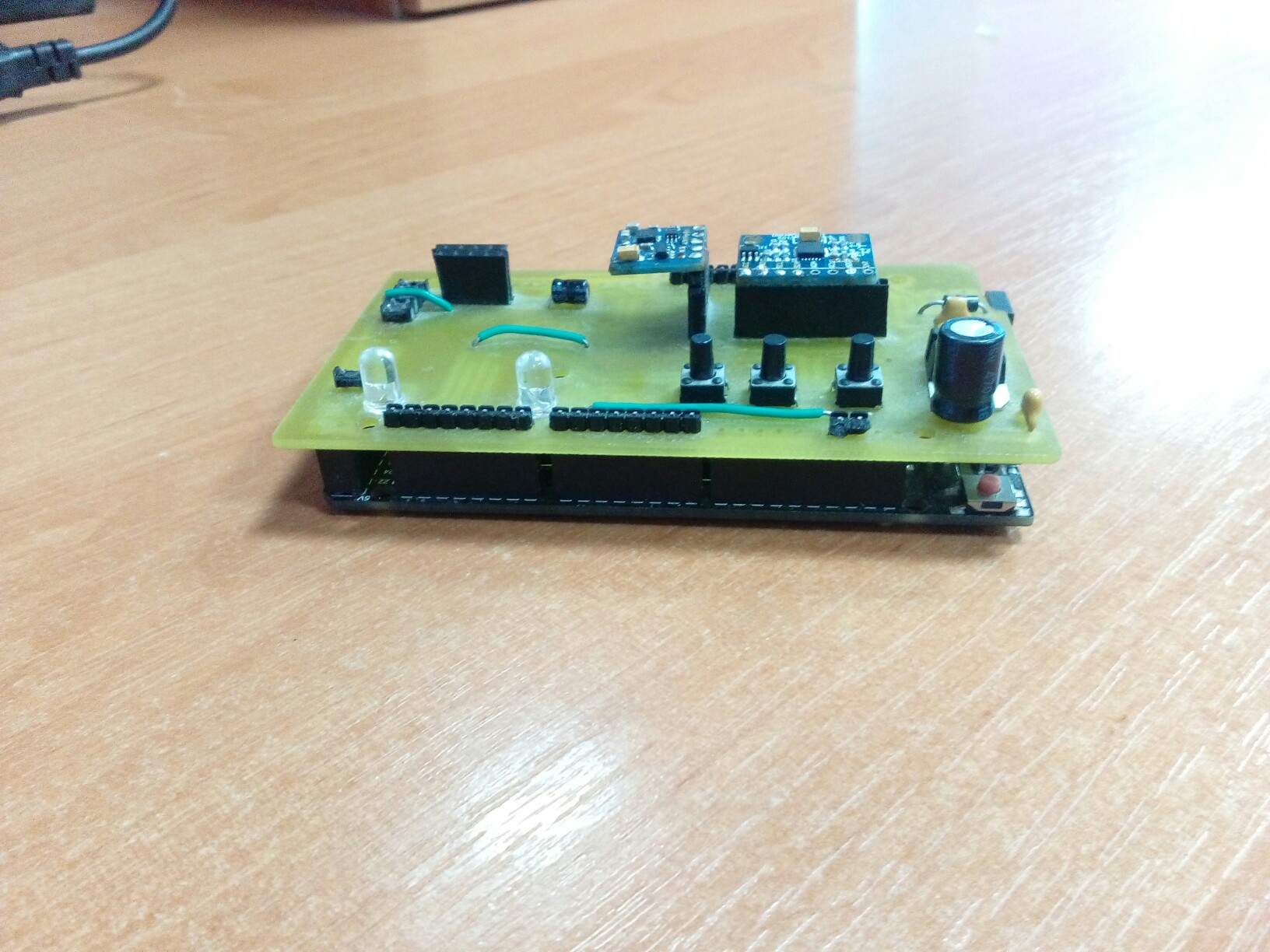
First, I designed a printed circuit board with the functionality I needed, on which I placed these three sensors. As a processing controller, I chose (or rather took what was) the Atmega2560 microcontroller. Sensors used common and cheap in the Chinese market. These are paired sensors triaxial gyroscope and accelerometer MPU6050 and magnetometer HMC5883l.



The algorithm for calculating the position in space is quite simple: first we determine the orientation in the form of the basis of the local coordinate system (LSC), which is associated with the sensors, and ultimately with the palm of the hand.



The orientation is determined relative to the initial coordinate system (NSC), which is essentially the initial position of the device at the time of power-up. The bases of the NSC and LSK consist of column vectors its ort:

$$

$$E_0 = \ left [\ vec {X} \ \ vec {Y} \ \ vec {Z} \ right] = \ left [\ begin {array} {cccc} 1 & 0 & 0 \\ 0 & 1 & 0 \\ 0 & 0 & 1 \ end {array} \ right] \\ E '= \ left [\ vec {x}' \ \ vec {y} '\ \ vec {z}' \ right]$$

They are related by:

$$

$$E '= CE_0$$

Where $$$C$ - transition matrix, it is the rotation matrix in space. The basis of the NSC will be considered the unit matrix. Consequently

$$

$$E '= C$$

.
After, the acceleration vector $$$\ vec {A}$ , which is known for LSK, must be defined in the NSC. This is done by multiplying the acceleration column vector by the basis of the FCS:

$$

$$\ vec {A} = E '\ vec {A}'$$

Then, the obtained acceleration vector is integrated twice in time and we get the distance, i.e. coordinates:

$$

$$\ vec {r} = \ iint \ vec {A} dt$$

The first attempts to implement this algorithm were very naive ... Naivety was that I found it possible only according to the gyroscope, using discrete integration, to obtain a rotation matrix around the axis. In this case, the axis can be viewed as an angular velocity pseudovector, whose components (projections on the axes) are the output data from the gyroscope sensor. And the angle in turn is obtained by integrating the modulus of the vector. The initial enthusiasm and enthusiasm disappeared when I saw a monstrous magnitude, the so-called “zero drift”, caused by a cumulative error due to discrete integration error and the sensor's own noise. Even then, I thought that according to the accelerometer, which at rest shows a vector opposite to the gravitational acceleration vector (hereinafter referred to as the gravity vector), the matrix can be adjusted, but here too there is uncertainty due to the fact that only up to a rotation of the angle around the Z axis. The correction will be complete if it is possible to restore the rotation matrix in an alternative way, i.e. without the use of gyro data.


Then it is necessary to use another factor by which it will be possible to make a full adjustment of the situation. This factor is the magnetic field of the Earth, which, along with gravity at a particular point on the planet, does not change with time (in the short term, of course). It is measured using the above-mentioned sensor HMC5883l. In this case, we have two vectors, which are sufficient to determine the position in space relative to them.

Now a natural question arises - “how to do it?”. After unsuccessful attempts to answer this questioning on my own, I got into the Internet, where I found the information I needed. The task of determining orientation in space according to three dimensions (angular velocity, gravity vector and magnetic field vector) also arises when designing amateur aircraft (for example, Copters), therefore this problem was not solved by various methods. One popular method is the so-called Majvik filter (Sebastian OH Madgwick). After reading the original article and not understanding Anglitsky, I turned to a wonderful translation (thanks to the author for the work done). While I was delving into studying the article, I had more and more thoughts about trying to write my own position filtering algorithm, considering that by this time my level of knowledge in this area had increased significantly. At least for the sake of interest "reinvent the wheel"! And I "invented" it. I give my reasoning below.

The algorithm uses the readings of all three sensors. Let me remind you, the task of the algorithm is the calculation of the orientation of the object and the compensation of the drift of the gyroscope zero, taking into account the given pairs of the accelerometer and the magnetometer. As a mathematical tool describing the position, the quaternion is used, since it is convenient in terms of construction and optimization of the algorithm and requires less mathematical operations to calculate it, unlike matrices. Quaternion rotation in space is as follows:

$$

$$q=\left[ q_1\ q_2\ q_3\ q_4 \right]$$

Knowing the axis of rotation described by the normalized vector $$$\vec{v}=\left[ v_x\ v_y\ v_z \right]$ and angle $$$\varphi$ (where they come from above) can be calculated quaternion:

$$

$$q_{v,\varphi}=\left[ \cos\left( \frac{\varphi}{2} \right)\ \ v_x\sin\left( \frac{\varphi}{2} \right)\ \ v_y\sin\left( \frac{\varphi}{2} \right)\ \ v_z\sin\left( \frac{\varphi}{2} \right) \right]\quad(*)$$

Then, using only the gyroscope readings, at each iteration of the cycle, we will calculate the current value of the quaternion by the expression:

$$

$$q_n^G=q_{n-1}q_{v,d\varphi}$$

Here $$$q_n^G$- quaternion at a given time. The index G above indicates that this value refers to the measured relative to the gyroscope readings, i.e. angular velocity;$$$q_{n-1}$ - the value of the quaternion at the previous time; $$$q_{v,d\varphi}$ –Change position for one step of measurement, we can say a discrete change of position by angle $$$d\varphi$ behind $$$dt$- the sampling period expressed by the rotation quaternion (*).

The next stage of calculation is finding the rotation matrix based on the data from a pair of accelerometer and magnetometer sensors. Specifically, we consider the gravity vector and the induction vector of the Earth’s magnetic field, which, as mentioned above, are static relative to the Earth and the associated NSC. Here the thesis is as follows: knowing the values ​​of gravity and induction in the basis of LSK and NSC, one can calculate the transition matrix (rotation) from NSC to LSK and the quaternion of rotation in space .

Denote by $$$\vec{G}$normalized initial gravity vector. It can be taken as follows:

$$

$$\vec{G}={\left[ 0\ 0\ 1 \right]}^T$$

Through $$$\vec{H}$ denote the normalized initial magnetic induction vector:

$$

$$\vec{H}={\left[ H_x\ H_y\ H_z \right]}^T$$

A third vector is also required. $$$\vec{K}$which is associated with these two. It is obtained by vector multiplication.$$$\vec{H}$ on $$$\vec{G}$ :

$$

$$\vec{K}={\left[ K_x\ K_y\ K_z \right]}^T= \vec{H}\times\vec{G}={\left[ H_y\ -H_x\ 0 \right]}^T$$

Now the matrix is ​​formed $$$M_0$which characterizes the initial position, i.e. NSC, since at the initial moment of time LSK coincides with the NSC. The matrix is ​​obtained from the components of the vectors$$$\vec{H}$ , $$$\vec{G}$ and $$$\vec{K}$ :

$$

$$M_0=\left[ \vec{H}\ \vec{G}\ \vec{K} \right]=\left[ \begin{array}{cccc} H_x&0&H_y\\H_y&0&-H_x\\H_z&1&0 \end{array} \right]$$

Similarly, but already at each iteration of the loop, a similar matrix is ​​created. $$$M'=\left[ \vec{h}\ \vec{g}\ \vec{k} \right]$ where $$$\vec{h}$ - current normalized vector of magnetic induction, $$$\vec{g}$ - current normalized gravity vector, $$$\vec{k} =\vec{h}\times\vec{g}$ .This matrix characterizes the position of the LSC, since these vectors are known in the coordinate system of the sensors, which coincides with the LCS. Then, knowing both matrices, we can write the following equation:

$$

$$E'M'=E_0M_0$$

It connects two matrices found under different circumstances. Given the expression$$$E'=CE_0$ and that basis $$$E_0$ - unit matrix, we get:

$$

$$CM'=M_0$$

Hence, we express the transition matrix $$$C$ :

$$

$$C={\left( M_0^{-1} \right)}^TM'^T$$

The first factor, as you can understand, is calculated only once at the very beginning of the algorithm, and does not require recalculation in the process. The second factor is formed quite easily and not forcedly at each iteration of the cycle.

After, when the transition matrix is ​​found, we transform it into a quaternion$$$q_n^A$(the algorithm for converting from matrix to quaternion is a public thing and I will not give it here).

As a result, we know two quaternions, found independently of each other. And to combine the results, I applied a simple complementary filter with a coefficient$$$F$ , which is taken from the range from 0 to 1:

$$

$$q_n=Fq_n^G+\left( 1-F \right)q_n^A$$

As a result, we obtain a quaternion, in which there is up-to-date information about the position in space of the device with the SINS module.

"Bicycle" went ... The algorithm worked, but in some positions it behaved somewhat inadequately, which in principle did not interfere, but also did not give reason to think about it positively. I have satisfied my sports interest, and now you can turn to ready-made, better-quality solutions. Then I returned to the article by Sebastian Majvik and decided to use his algorithm, the good thing is that this wonderful person published all the sources on the project website. The archive contained source codes in various languages, including the Matlab language. This fact influenced my decision to abandon the idea of ​​doing all the calculations on a microcontroller (especially since it is 8-bit) and write the program already on a computer in Matlab. The microcontroller is used only for interrogating sensors and sending data to a PC (a similar situation with a manipulator). In this case, the main program code, which is subject to changes and debugging, is based on Matlab, which is very convenient in the process.

Well, we got the orientation given by the quaternion. What's next for the plan? And then follows the finding of the linear coordinates of the object according to the accelerometer. Well, here it is better to simply state that it is impossible to determine the coordinates with the required accelerometer accuracy. Even at least find a change of position that would be adequate! Of course, there were attempts to solve this problem, but it was impossible to find coordinates in real time. Why? Because the double discrete integration of noisy sensor readings led only to flight into the stratosphere, and at a breakneck speed, but not at all to a positive result. Therefore, I have cut off the algorithm indicated at the beginning of the paragraph until the orientation is found, and stopped at this.

3. Everything else

So, here I am getting close to the final design stage, having played enough with the manipulator and screwed on the IMU-sensor. Working on the two previous stages, I had a clear idea of ​​how everything will work and by what algorithm. Therefore, I dealt with this stage rather quickly. Since only the orientation of the palm is known, we work directly with the working body that needs to be oriented accordingly. The RO can take any direction, if it does not violate the working area (it does not turn out all 360).

In the paragraph about the development of the manipulator, the vector RO was set manually, and afterwards there were angles of rotation of the drives. So, this vector should be determined based on the orientation of the palm of the hand. Orientation can be expressed as a basis $$$E '$ by finding it, converting the quaternion into a matrix. The basis consists of its column vectors ort, therefore we get three vectors $$$\ vec {x} '$ , $$$\ vec {y} '$ and $$$\ vec {z} '$ . It will be convenient to take RO vector for orientation. $$$\ vec {x} '$ as I assumed such initial position of the manipulator, when all the links and PO are located in the XZ plane of the base coordinate system, and the PO at this moment is horizontal, i.e. vector $$$\ vec {v_0}$ at the beginning, it is aligned with the X axis of the BSC and the NSC (the initial position of the BINS module is positioned so that the NSC coincides with the BSC of the manipulator). In this case, the first column of the matrix $$$E '$ equate to vector $$$\ vec {v_0}$ . After normalizing it along the length of the PO, we obtain the required vector relative to the base coordinate system of the manipulator. Then we follow the sequence of calculating the generalized coordinates from item 1.

It should be noted that the manipulator, when changing the orientation of the PO, is able to perform movement in two modes: the first is when the flange point is stationary, the second is when the end point of the PO is stationary, but its orientation is observed. The second mode is more interesting because even in the absence of linear movement, all the axes of rotation are still involved to move the flange point, while at the same time observing the orientation of the PO. However, the transition from the first mode to the second occurs with the addition of only one operation of vector subtraction to find the vector $$$\ vec {r}$ (see paragraph 1).

All the above operations were also programmed in the Matlab environment. In general, the structure of the program is as follows:

1. Calibration on startup. We set up the entire farm to its original position and, not daring to touch, calibrate the SINS module with a certain amount of raw data from it. Calibration is necessary, because you need to remove the initial offset, which gave the filter (I did not understand why, and so it worked perfectly).
2. The beginning of the script. We initialize all libraries and variables, set the initial position of the flange or end point PO.
3. Run a cycle. At each iteration, we query the sensors, find the quaternion, translate it into a matrix, which is the basis $$$E '$ , it is the basis in which the RO is located. The first column is taken as the orientation of the PO and we find all the generalized coordinates using the mathematical considerations from paragraph 1.
4. Knowing the generalized coordinates at the last moment of time and at the present, we calculate the angular velocity of rotation of the axes.
5. We send the data packet to the manipulator microcontroller.

It turned out of course koryavenko, but if you look, you can see a positive result of the study. This work, of course, does not pretend to be completed and requires a lot of effort for refinement, but only if this can be applied. But I have not yet found a specific application ... Can someone tell me?