"There and back" for neural networks, or a review of auto-encoder applications in text analysis
We have already written in the very first article of our corporate blog about how the algorithm for detecting transferable borrowings works. Only a couple of paragraphs in that article are devoted to the topic of text comparison, although the idea is worthy of a much more detailed description. However, as you know, it is impossible to tell everything at once, although I really want to. In an attempt to pay tribute to this topic and the network architecture called “ auto-encoder ”, to which we have very warm feelings, we with Oleg_Bakhteev wrote this review.

Source: Deep Learning for NLP (without Magic)
As we mentioned in that article, we had a “semantic” comparison of the texts - we compared not the text fragments themselves, but the vectors corresponding to them. Such vectors were obtained as a result of training of the neural network, which displayed a text fragment of an arbitrary length into a vector of large but fixed dimension. How to get such a mapping and how to teach the network to produce the desired results is a separate question, which will be discussed below.
Formally, an autocoder (or autoencoder) is a neural network that trains to reconstruct objects that are taken to the input of the network.
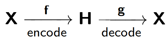
The autocoder consists of two parts: the encoder f , which encodes the sample X into its internal representation H , and the decoder g , which restores the original sample. Thus, the auto-encoder tries to combine the restored version of each sample object with the original object.
')
When training autocoder minimizes the following function:
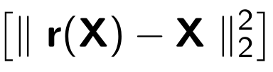
Where r is the recovered version of the original object:

Consider an example presented in blog.keras.io :

The network receives object x as an input (in our case, the number 2).
Our network encodes this object in a hidden state. Then, the reconstruction of the object r , which should be similar to x, is reconstructed from the hidden state. As we can see, the restored image (on the right) has become more blurred. This is explained by the fact that we try to save in the hidden view only the most important features of the object, so the object is restored with losses.
The autocoder model is trained on the basis of a damaged phone, where one person (encoder) transmits information (x ) to the second person (decoder ) , and the latter, in turn, tells it to the third person (r (x)) .
One of the main purposes of such autocoders is to reduce the dimension of the original space. When we deal with auto-encoders, the neural network training procedure itself forces the auto-encoder to memorize the main features of the objects, which will make it easier to restore the original objects of the sample.
Here we can draw an analogy with the method of principal components : this is the method of reducing the dimension, the result of which is the projection of the sample onto the subspace in which the dispersion of this sample is maximal.
Indeed, the auto-encoder is a generalization of the principal component method: in the case where we restrict ourselves to considering linear models, the auto-encoder and the principal component method give the same vector representations. The difference arises when we consider more complex models, for example, multilayer fully connected neural networks, as an encoder and a decoder.
An example of comparing the principal component method and the auto-encoder is presented in the article Reducing the Dimensionality of Data with Neural Networks :
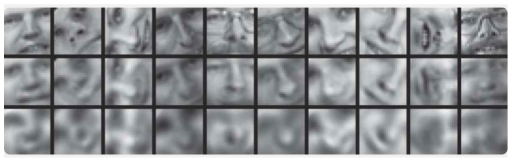
It demonstrates the results of auto-encoder training and the principal component method for sampling images of human faces. The first line shows the faces of people from the control sample, i.e. from the specially deferred part of the sample that was not used by the algorithms in the learning process. The second and third lines contain the recovered images from the hidden states of the autocoder and the principal component method, respectively, of the same dimension. It is clearly seen how much better the auto-encoder worked.
In the same article, another illustrative example: a comparison of the results of the work of the auto-encoder and the LSA method for the task of information retrieval. The LSA method, like the principal component method, is a classical machine learning method and is often used in tasks related to the processing of natural language.

The figure shows a 2D projection of a set of documents obtained using the auto-encoder and the LSA method. Colors indicate the subject of the document. It can be seen that the projection from the auto-encoder well breaks the documents by topic, while the LSA gives a much more noisy result.
Another important use of autocoders is the pre-training of networks . Network pre-training is used when the network being optimized is deep enough. In this case, training the network from scratch can turn out to be quite complex, so first the entire network is represented as a chain of encoders.
The pre-learning algorithm is quite simple: for each layer, we train our auto-encoder, and then we ask that the output of the next encoder is at the same time the input for the next layer of the network. The resulting model consists of a chain of encoders, trained to eagerly preserve the most important features of objects, each on its own layer. The pre-training scheme is presented below:
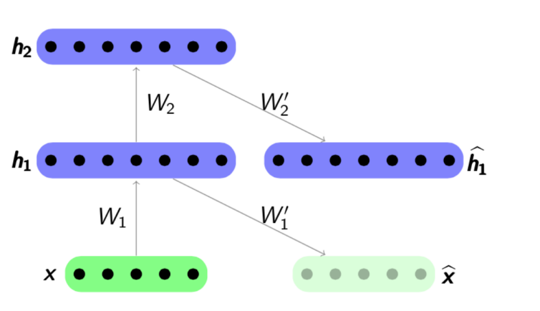
Source: psyyz10.imtqy.com
Such a structure is called Stacked Autoencoder and is often used as “overclocking” for further learning of the complete deep network model. The motivation for such learning of a neural network is that a deep neural network is a nonconvex function: in the process of learning a network, the optimization of parameters can “get stuck” in a local minimum. The greedy pre-training of network parameters allows you to find a good starting point for final training and thus try to avoid such local minima.
Of course, we have considered far from all possible structures, as there are still Sparse Autoencoders , Denoising Autoencoders , Contractive Autoencoder , Reconstruction Contractive Autoencoder . They differ from each other using different error functions and penalty terms to them. All these architectures, we think, are worthy of a separate review. In our article, we first of all show the general concept of auto-encoders and those specific tasks of text analysis that are solved with its use.
We now turn to specific examples of the use of autocoders for text analysis problems. We are interested in both sides of the application - both models for obtaining internal representations, and using these internal representations as attributes, for example, in the further task of classification. Articles on this topic most often affect such tasks as sentiment analysis, or detection of paraphrases, but there are also works describing the use of autocoders for comparing texts in different languages or for machine translation.
In the tasks of text analysis, the most frequent object is the sentence, i.e. ordered sequence of words. Thus, the autocoder takes on input this particular sequence of words, or rather, vector representations of these words, taken from some pre-trained model. What is the vector representation of words, was considered on Habré in some detail, for example, here . Thus, the auto-encoder, taking as input a sequence of words, should train some internal representation of the entire sentence, corresponding to those characteristics that are important to us, based on the task. In the problems of text analysis, we need to map the sentences into vectors so that they are close in the sense of some distance function, most often a cosine measure:
Source: Deep Learning for NLP (without Magic)
One of the first authors who showed the successful use of autocoders in text analysis was Richard Socher .
In his article Dynamic Pooling and Unfolding Recursive Autoencoders for Paraphrase Detection, he describes a new autocoder structure - Unfolding Recursive Autoencoder (Unfolding RAE) (see the figure below).

Unfolding rae
It is assumed that the sentence structure is defined by the syntax parser . The simplest structure is considered - the structure of a binary tree. Such a tree consists of leaves - words of a fragment, internal nodes (branch nodes) - phrases, and a terminal vertex. Taking the input sequence of words (x 1 , x 2 , x 3 ) (the three vector representations of words in this example), the autocoder sequentially encodes, in this case, right-to-left, the vector representations of the words into vector representations of word combinations, and then into presentation of the whole sentence. Specifically, in this example, we first associate the vectors x 2 and x 3 , then multiply them by the matrix W e having the dimension of hidden × 2visible , where hidden is where the size of the hidden internal representation, visible is the dimension of the word vector. Thus, we reduce the dimension, then adding non-linearity using the tanh function. In the first step, we get a hidden vector representation for the phrase two words x 2 and x 3 : h 1 = tanh (W e [x 2 , x 3 ] + b e ) . In the second, we merge it and the remaining word h 2 = tanh (W e [h 1 , x 1 ] + b e ) and get a vector representation for the entire sentence — h 2 . As mentioned above, in the definition of the auto-encoder, we need to minimize the error between objects and their restored versions. In our case, these are words. Therefore, having obtained the final vector representation of the entire sentence h 2 , we decode its restored versions (x 1 ', x 2 ', x 3 '). The decoder here works on the same principle as the encoder, only the matrix of parameters and the shift vector are different: W d and b d .
Using the structure of a binary tree, it is possible to encode sentences of any length into a vector of fixed dimension - we always combine over a pair of vectors of the same dimension using the same matrix of parameters W e . In the case of a non-binary tree, you just need to initialize the matrices in advance for the cases if we want to combine more than two words - 3, 4, ... n, in this case, the matrix will simply have the dimension of hidden × invisible .
It is noteworthy that in this article, the trained vector representations of phrases are used not only to solve the problem of classification - whether or not a couple of sentences are paraphrased. Experimental data on the search for the nearest neighbors are also given - based only on the received vector of the proposal, the nearest ones in the sample of the vector are found for it, which are close to it in meaning:

However, no one bothers us to use for the consistent combination of words in a sentence and other network architectures for encoding and decoding.
Here is an example from the article NIPS 2017 - Deconvolutional Paragraph Representation Learning :

We see that encoding sample X into a hidden representation of h occurs using a convolutional neural network , and the decoder works in the same way.
Or here’s an example using GRU-GRU in the Skip-Thought Vectors article.
An interesting feature here is that the model works with triples of sentences: ( s i-1 , s i , s i + 1 ). The sentence s i is encoded using the standard GRU formulas, and the decoder, using information about the internal representation s i , attempts to decode s i-1 and s i + 1 , also using GRU.

The principle of operation in this case resembles the standard model of neural network machine translation , which operates according to the encoder-decoder scheme. However, here we do not have two languages, we feed a phrase in one language to the input of our coding block, and we are trying to restore it. In the process of learning, there is a minimization of some internal functional quality (this is not always a reconstruction error), then, if required, the pre-trained vectors are used as attributes in another task.
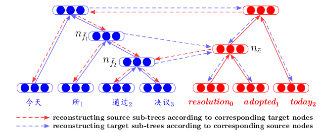
In another work - Bilingual Correspondence Recursive Autoencoders for the Statistical Machine Translation - an architecture is presented that allows you to take a fresh look at machine translation. First, recursive autocoders are taught separately for two languages (according to the principle described above, where Unfolding RAE was introduced). Then, between them, the third autoencoder is trained - a mapping between two languages. This architecture has a clear advantage - when displaying texts in different languages into one common hidden space, we can compare them, without using machine translation, as an intermediate step.
Pre-training autocoders on text fragments is often found in ranking training articles. Here, again, it is important that, in order to train the final ranking quality functional, we first pre-train the autocoder to better initialize the request and response vectors to the network input.

And, of course, we cannot but mention Variational autocoders ( Variational Autoencoders , or VAE) as generative models. Best of all, of course, just watch this lecture entry from Yandex . It is enough for us to say the following: if we want to generate objects from the hidden space of a conventional auto-encoder, the quality of such generation will be low, since we know nothing about the distribution of the hidden variable. But you can immediately train the auto-encoder for generation, introducing the distribution assumption.
And then, using VAE, you can generate texts from this hidden space, for example, as the authors of the article Generating Sentences from a Continuous Space or A Hybrid Convolutional Variational Autoencoder for Text Generation do .
The VAE generative properties are also well manifested in the task of comparing texts in different languages - A Variational Autoencoding Approach for Inducing Cross-lingual Word Embeddings is a great example.
As an output, we want to make a small forecast. Representation Learning - training internal presentations using VAE specifically, in conjunction with Generative Adversarial Networks , is one of the most evolving approaches in recent years - this can be judged by the most frequent topics of articles at the latest top machine learning conferences ICLR 2018 and ICML 2018 . This is quite logical - because its use has helped raise the quality in a number of tasks, and not only related to texts. But this is a completely different review topic ...
Source: Deep Learning for NLP (without Magic)
As we mentioned in that article, we had a “semantic” comparison of the texts - we compared not the text fragments themselves, but the vectors corresponding to them. Such vectors were obtained as a result of training of the neural network, which displayed a text fragment of an arbitrary length into a vector of large but fixed dimension. How to get such a mapping and how to teach the network to produce the desired results is a separate question, which will be discussed below.
What is an auto encoder?
Formally, an autocoder (or autoencoder) is a neural network that trains to reconstruct objects that are taken to the input of the network.
The autocoder consists of two parts: the encoder f , which encodes the sample X into its internal representation H , and the decoder g , which restores the original sample. Thus, the auto-encoder tries to combine the restored version of each sample object with the original object.
')
When training autocoder minimizes the following function:
Where r is the recovered version of the original object:
Consider an example presented in blog.keras.io :
The network receives object x as an input (in our case, the number 2).
Our network encodes this object in a hidden state. Then, the reconstruction of the object r , which should be similar to x, is reconstructed from the hidden state. As we can see, the restored image (on the right) has become more blurred. This is explained by the fact that we try to save in the hidden view only the most important features of the object, so the object is restored with losses.
The autocoder model is trained on the basis of a damaged phone, where one person (encoder) transmits information (x ) to the second person (decoder ) , and the latter, in turn, tells it to the third person (r (x)) .
One of the main purposes of such autocoders is to reduce the dimension of the original space. When we deal with auto-encoders, the neural network training procedure itself forces the auto-encoder to memorize the main features of the objects, which will make it easier to restore the original objects of the sample.
Here we can draw an analogy with the method of principal components : this is the method of reducing the dimension, the result of which is the projection of the sample onto the subspace in which the dispersion of this sample is maximal.
Indeed, the auto-encoder is a generalization of the principal component method: in the case where we restrict ourselves to considering linear models, the auto-encoder and the principal component method give the same vector representations. The difference arises when we consider more complex models, for example, multilayer fully connected neural networks, as an encoder and a decoder.
An example of comparing the principal component method and the auto-encoder is presented in the article Reducing the Dimensionality of Data with Neural Networks :
It demonstrates the results of auto-encoder training and the principal component method for sampling images of human faces. The first line shows the faces of people from the control sample, i.e. from the specially deferred part of the sample that was not used by the algorithms in the learning process. The second and third lines contain the recovered images from the hidden states of the autocoder and the principal component method, respectively, of the same dimension. It is clearly seen how much better the auto-encoder worked.
In the same article, another illustrative example: a comparison of the results of the work of the auto-encoder and the LSA method for the task of information retrieval. The LSA method, like the principal component method, is a classical machine learning method and is often used in tasks related to the processing of natural language.
The figure shows a 2D projection of a set of documents obtained using the auto-encoder and the LSA method. Colors indicate the subject of the document. It can be seen that the projection from the auto-encoder well breaks the documents by topic, while the LSA gives a much more noisy result.
Another important use of autocoders is the pre-training of networks . Network pre-training is used when the network being optimized is deep enough. In this case, training the network from scratch can turn out to be quite complex, so first the entire network is represented as a chain of encoders.
The pre-learning algorithm is quite simple: for each layer, we train our auto-encoder, and then we ask that the output of the next encoder is at the same time the input for the next layer of the network. The resulting model consists of a chain of encoders, trained to eagerly preserve the most important features of objects, each on its own layer. The pre-training scheme is presented below:
Source: psyyz10.imtqy.com
Such a structure is called Stacked Autoencoder and is often used as “overclocking” for further learning of the complete deep network model. The motivation for such learning of a neural network is that a deep neural network is a nonconvex function: in the process of learning a network, the optimization of parameters can “get stuck” in a local minimum. The greedy pre-training of network parameters allows you to find a good starting point for final training and thus try to avoid such local minima.
Of course, we have considered far from all possible structures, as there are still Sparse Autoencoders , Denoising Autoencoders , Contractive Autoencoder , Reconstruction Contractive Autoencoder . They differ from each other using different error functions and penalty terms to them. All these architectures, we think, are worthy of a separate review. In our article, we first of all show the general concept of auto-encoders and those specific tasks of text analysis that are solved with its use.
How does this work in lyrics?
We now turn to specific examples of the use of autocoders for text analysis problems. We are interested in both sides of the application - both models for obtaining internal representations, and using these internal representations as attributes, for example, in the further task of classification. Articles on this topic most often affect such tasks as sentiment analysis, or detection of paraphrases, but there are also works describing the use of autocoders for comparing texts in different languages or for machine translation.
In the tasks of text analysis, the most frequent object is the sentence, i.e. ordered sequence of words. Thus, the autocoder takes on input this particular sequence of words, or rather, vector representations of these words, taken from some pre-trained model. What is the vector representation of words, was considered on Habré in some detail, for example, here . Thus, the auto-encoder, taking as input a sequence of words, should train some internal representation of the entire sentence, corresponding to those characteristics that are important to us, based on the task. In the problems of text analysis, we need to map the sentences into vectors so that they are close in the sense of some distance function, most often a cosine measure:
Source: Deep Learning for NLP (without Magic)
One of the first authors who showed the successful use of autocoders in text analysis was Richard Socher .
In his article Dynamic Pooling and Unfolding Recursive Autoencoders for Paraphrase Detection, he describes a new autocoder structure - Unfolding Recursive Autoencoder (Unfolding RAE) (see the figure below).
Unfolding rae
It is assumed that the sentence structure is defined by the syntax parser . The simplest structure is considered - the structure of a binary tree. Such a tree consists of leaves - words of a fragment, internal nodes (branch nodes) - phrases, and a terminal vertex. Taking the input sequence of words (x 1 , x 2 , x 3 ) (the three vector representations of words in this example), the autocoder sequentially encodes, in this case, right-to-left, the vector representations of the words into vector representations of word combinations, and then into presentation of the whole sentence. Specifically, in this example, we first associate the vectors x 2 and x 3 , then multiply them by the matrix W e having the dimension of hidden × 2visible , where hidden is where the size of the hidden internal representation, visible is the dimension of the word vector. Thus, we reduce the dimension, then adding non-linearity using the tanh function. In the first step, we get a hidden vector representation for the phrase two words x 2 and x 3 : h 1 = tanh (W e [x 2 , x 3 ] + b e ) . In the second, we merge it and the remaining word h 2 = tanh (W e [h 1 , x 1 ] + b e ) and get a vector representation for the entire sentence — h 2 . As mentioned above, in the definition of the auto-encoder, we need to minimize the error between objects and their restored versions. In our case, these are words. Therefore, having obtained the final vector representation of the entire sentence h 2 , we decode its restored versions (x 1 ', x 2 ', x 3 '). The decoder here works on the same principle as the encoder, only the matrix of parameters and the shift vector are different: W d and b d .
Using the structure of a binary tree, it is possible to encode sentences of any length into a vector of fixed dimension - we always combine over a pair of vectors of the same dimension using the same matrix of parameters W e . In the case of a non-binary tree, you just need to initialize the matrices in advance for the cases if we want to combine more than two words - 3, 4, ... n, in this case, the matrix will simply have the dimension of hidden × invisible .
It is noteworthy that in this article, the trained vector representations of phrases are used not only to solve the problem of classification - whether or not a couple of sentences are paraphrased. Experimental data on the search for the nearest neighbors are also given - based only on the received vector of the proposal, the nearest ones in the sample of the vector are found for it, which are close to it in meaning:
However, no one bothers us to use for the consistent combination of words in a sentence and other network architectures for encoding and decoding.
Here is an example from the article NIPS 2017 - Deconvolutional Paragraph Representation Learning :
We see that encoding sample X into a hidden representation of h occurs using a convolutional neural network , and the decoder works in the same way.
Or here’s an example using GRU-GRU in the Skip-Thought Vectors article.
An interesting feature here is that the model works with triples of sentences: ( s i-1 , s i , s i + 1 ). The sentence s i is encoded using the standard GRU formulas, and the decoder, using information about the internal representation s i , attempts to decode s i-1 and s i + 1 , also using GRU.
The principle of operation in this case resembles the standard model of neural network machine translation , which operates according to the encoder-decoder scheme. However, here we do not have two languages, we feed a phrase in one language to the input of our coding block, and we are trying to restore it. In the process of learning, there is a minimization of some internal functional quality (this is not always a reconstruction error), then, if required, the pre-trained vectors are used as attributes in another task.
In another work - Bilingual Correspondence Recursive Autoencoders for the Statistical Machine Translation - an architecture is presented that allows you to take a fresh look at machine translation. First, recursive autocoders are taught separately for two languages (according to the principle described above, where Unfolding RAE was introduced). Then, between them, the third autoencoder is trained - a mapping between two languages. This architecture has a clear advantage - when displaying texts in different languages into one common hidden space, we can compare them, without using machine translation, as an intermediate step.
Pre-training autocoders on text fragments is often found in ranking training articles. Here, again, it is important that, in order to train the final ranking quality functional, we first pre-train the autocoder to better initialize the request and response vectors to the network input.
And, of course, we cannot but mention Variational autocoders ( Variational Autoencoders , or VAE) as generative models. Best of all, of course, just watch this lecture entry from Yandex . It is enough for us to say the following: if we want to generate objects from the hidden space of a conventional auto-encoder, the quality of such generation will be low, since we know nothing about the distribution of the hidden variable. But you can immediately train the auto-encoder for generation, introducing the distribution assumption.
And then, using VAE, you can generate texts from this hidden space, for example, as the authors of the article Generating Sentences from a Continuous Space or A Hybrid Convolutional Variational Autoencoder for Text Generation do .
The VAE generative properties are also well manifested in the task of comparing texts in different languages - A Variational Autoencoding Approach for Inducing Cross-lingual Word Embeddings is a great example.
As an output, we want to make a small forecast. Representation Learning - training internal presentations using VAE specifically, in conjunction with Generative Adversarial Networks , is one of the most evolving approaches in recent years - this can be judged by the most frequent topics of articles at the latest top machine learning conferences ICLR 2018 and ICML 2018 . This is quite logical - because its use has helped raise the quality in a number of tasks, and not only related to texts. But this is a completely different review topic ...
Source: https://habr.com/ru/post/418173/
All Articles