Text analysis using convolutional neural networks

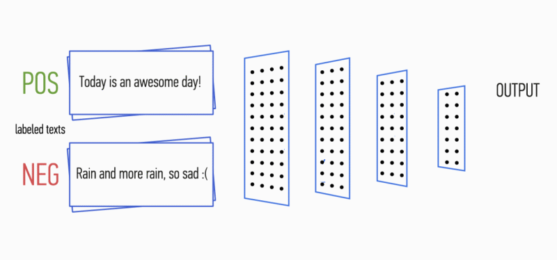
Imagine that you have a paragraph of text. Is it possible to understand what kind of emotion this text carries: joy, sadness, anger? Can. Simplify your task and we will classify the emotion as positive or negative, without clarification. There are many ways to solve such a problem, and one of them is convolutional neural networks (Convolutional Neural Networks). CNN was originally developed for image processing, but they successfully cope with the solution of problems in the field of automatic text processing. I will introduce you to the binary analysis of the tonality of Russian-language texts using the convolutional neural network, for which the vector representations of words were formed on the basis of the trained Word2Vec model.

The article is an overview, I focused on the practical component. And at once I want to warn you that decisions made at each stage may not be optimal. Before reading, I recommend reading the introductory article on the use of CNN in problems of processing natural languages, as well as to read the material about the methods of vector representation of words.

Architecture

The considered CNN architecture is based on approaches [1] and [2]. The approach [1], which uses the ensemble of convolutional and recurrent networks, at the largest annual competition in computational linguistics SemEval-2017 won first places [3] in five nominations in the task for analyzing the tonality of Task 4 .
')

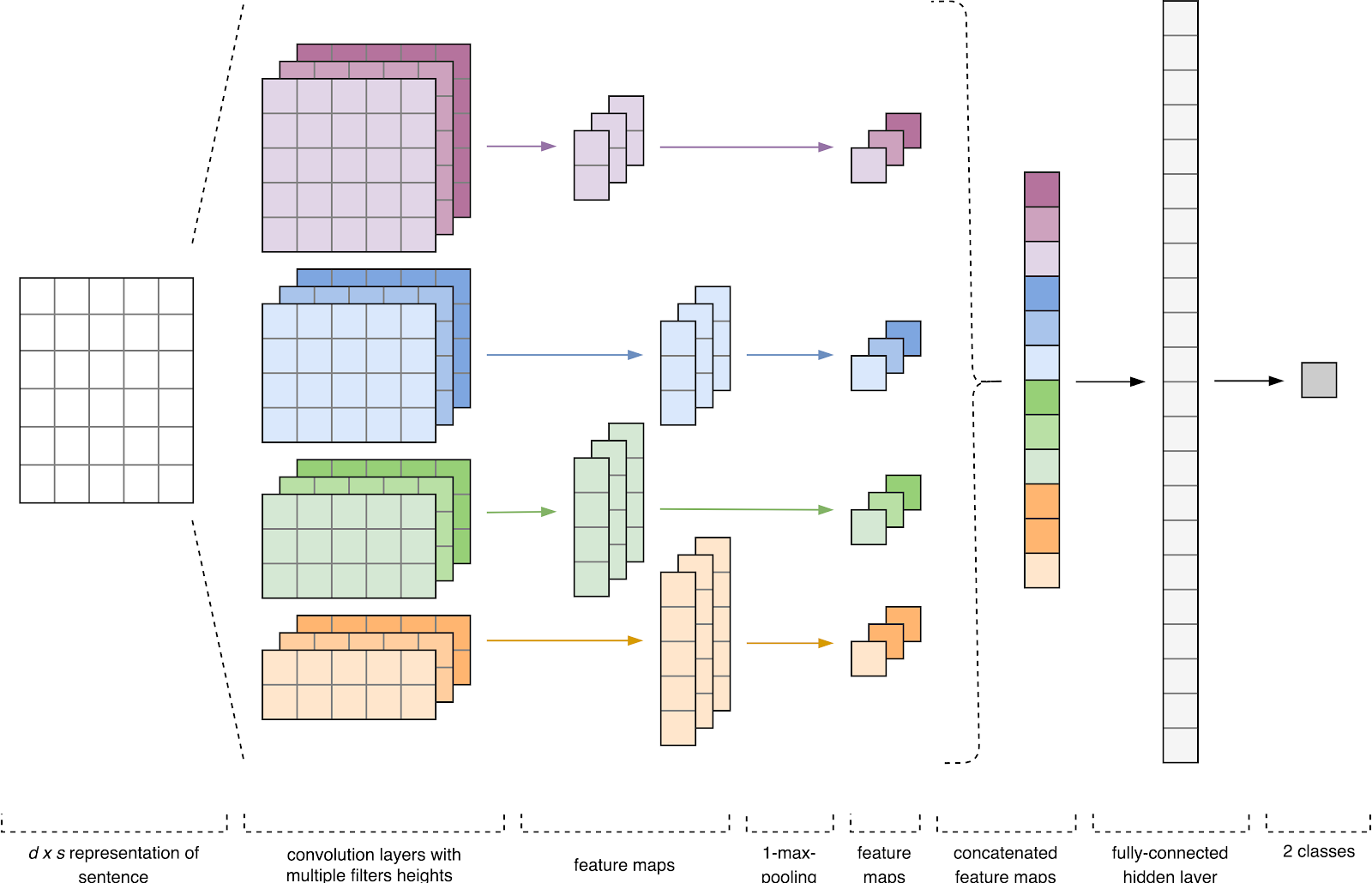
Figure 1. CNN architecture [2].

The input data of CNN (Fig. 1) is a matrix with a fixed height n , where each row is a vector map of the token to the attribute space of dimension k . Distributive semantics tools such as Word2Vec, Glove, FastText, etc. are often used to form feature spaces.

At the first stage, the input matrix is ​​processed by convolution layers. As a rule, filters have a fixed width equal to the dimension of the attribute space, and for filtering the filters only one parameter is adjusted - height h . It turns out that h is the height of adjacent rows, considered by the filter together. Accordingly, the dimension of the output matrix of attributes for each filter varies depending on the height of this filter h and the height of the original matrix n .

Further, the feature map obtained at the output of each filter is processed by a sub-sampling layer with a specific compression function (in the image - 1-max pooling), i.e. reduces the dimension of the generated feature map. This extracts the most important information for each convolution, regardless of its position in the text. In other words, for the used vector display, the combination of convolution layers and sub-sampling layers allows to extract the most significant n- programs from the text.

After this, feature maps calculated at the output of each layer of sub-sampling are combined into one common feature vector. It is fed to the input of the hidden fully meshed layer, and then it goes to the output layer of the neural network, where the total marks of the classes are calculated.

Data for training

For learning, I chose the corpus of short texts by Yulia Rubtsova , formed on the basis of Russian-language messages from Twitter [4]. It contains 114,991 positive, 111,923 negative tweets, as well as a database of untagged tweets with a volume of 17,639,674 posts.

import pandas as pd import numpy as np #   n = ['id', 'date', 'name', 'text', 'typr', 'rep', 'rtw', 'faw', 'stcount', 'foll', 'frien', 'listcount'] data_positive = pd.read_csv('data/positive.csv', sep=';', error_bad_lines=False, names=n, usecols=['text']) data_negative = pd.read_csv('data/negative.csv', sep=';', error_bad_lines=False, names=n, usecols=['text']) #    sample_size = min(data_positive.shape[0], data_negative.shape[0]) raw_data = np.concatenate((data_positive['text'].values[:sample_size], data_negative['text'].values[:sample_size]), axis=0) labels = [1] * sample_size + [0] * sample_size 

Before the beginning of the training, the texts underwent the preliminary processing procedure:

• lower case;
  
• substitution of “e” for “e”;
  
• replacement of links to the token "URL";
  
• replacing the user reference to the token "USER";
  
• deletion of punctuation marks.
  

 import re def preprocess_text(text): text = text.lower().replace("", "") text = re.sub('((www\.[^\s]+)|(https?://[^\s]+))', 'URL', text) text = re.sub('@[^\s]+', 'USER', text) text = re.sub('[^a-zA-Z--1-9]+', ' ', text) text = re.sub(' +', ' ', text) return text.strip() data = [preprocess_text(t) for t in raw_data] 

Next, I broke the data set into a training and test sample in a 4: 1 ratio.

 from sklearn.model_selection import train_test_split x_train, x_test, y_train, y_test = train_test_split(data, labels, test_size=0.2, random_state=1) 

Vector word mapping

The input data of a convolutional neural network is a matrix with a fixed height n , where each row is a vector mapping of a word to a feature space of dimension k . To form the embedding layer of the neural network, I used the Word2Vec [5] distributive semantics utility, designed to map the semantic meaning of words into vector space. Word2Vec finds relationships between words according to the assumption that in similar contexts there are semantically close words. More information about Word2Vec can be found in the original article , as well as here and here . Since tweets are characterized by author's punctuation and emoticons, defining the boundaries of sentences becomes quite a laborious task. In this paper, I assumed that each tweet contains only one sentence.

The database of unmarked tweets is stored in SQL format and contains more than 17.5 million records. For convenience, I converted it to SQLite using this script.

 import sqlite3 #  SQLite   conn = sqlite3.connect('mysqlite3.db') c = conn.cursor() with open('data/tweets.txt', 'w', encoding='utf-8') as f: #    for row in c.execute('SELECT ttext FROM sentiment'): if row[0]: tweet = preprocess(row[0]) #      print(tweet, file=f) 

Then, using the Gensim library, I trained the Word2Vec-model with the following parameters:

• size = 200 is the dimension of the attribute space;
  
• window = 5 - the number of words from the context that the algorithm analyzes;
  
• min_count = 3 - the word must occur at least three times for the model to take it into account.
  

 import logging import multiprocessing import gensim from gensim.models import Word2Vec logging.basicConfig(format='%(asctime)s : %(levelname)s : %(message)s', level=logging.INFO) #      data = gensim.models.word2vec.LineSentence('data/tweets.txt') #   model = Word2Vec(data, size=200, window=5, min_count=3, workers=multiprocessing.cpu_count()) model.save("models/w2v/model.w2v") 

Figure 2. Visualization of clusters of similar words using t-SNE.

For a more detailed understanding of the work of Word2Vec in Fig. Figure 2 shows the visualization of several clusters of similar words from a trained model mapped into a two-dimensional space using the t-SNE visualization algorithm .

Vector text display

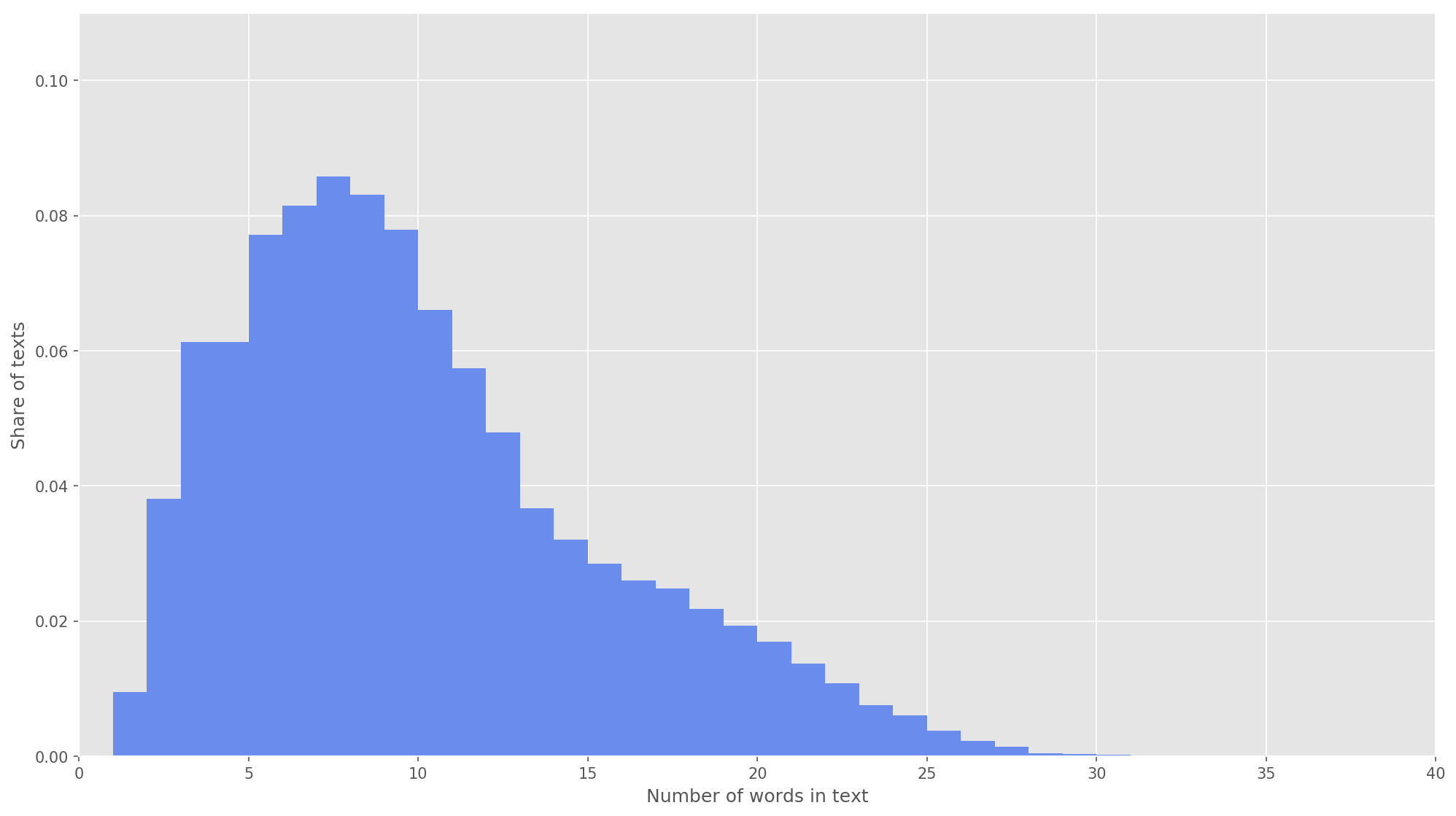
Figure 3. The length distribution of texts.

In the next step, each text was mapped to an array of token identifiers. I chose the dimension of the text vector s = 26 , since, with this value, 99.71% of all texts in the formed package are fully covered (Fig. 3). If, during the analysis, the number of words in the tweet exceeded the height of the matrix, the remaining words were discarded and not considered in the classification. The total dimension of the matrix of the sentence was s × d = 26 × 200 .

 from keras.preprocessing.text import Tokenizer from keras.preprocessing.sequence import pad_sequences #   (    ) SENTENCE_LENGTH = 26 #   NUM = 100000 def get_sequences(tokenizer, x): sequences = tokenizer.texts_to_sequences(x) return pad_sequences(sequences, maxlen=SENTENCE_LENGTH) # C    tokenizer = Tokenizer(num_words=NUM) tokenizer.fit_on_texts(x_train) #        x_train_seq = get_sequences(tokenizer, x_train) x_test_seq = get_sequences(tokenizer, x_test) 

Convolutional neural network

To build a neural network, I used the Keras library, which is a high-level superstructure over TensorFlow, CNTK and Theano. Keras has excellent documentation as well as a blog that covers many of the tasks of machine learning, for example, embedding layer initialization . In our case, the embedding-layer was initiated by the weights obtained during the training Word2Vec. To minimize changes in the embedding layer, I froze it during the first stage of training.

 from keras.layers import Input from keras.layers.embeddings import Embedding tweet_input = Input(shape=(SENTENCE_LENGTH,), dtype='int32') tweet_encoder = Embedding(NUM, DIM, input_length=SENTENCE_LENGTH, weights=[embedding_matrix], trainable=False)(tweet_input) 

In the developed architecture, filters with heights h = (2, 3, 4, 5) are used, which are intended for parallel processing of digrams, trigrams, 4-grams and 5-grams, respectively. I added 10 convolutional layers for each height of the filter to the neural network, the activation function is ReLU. Recommendations on finding the optimal height and number of filters can be found in [2].

After processing by the convolution layers, the feature maps arrived at the subsampling layers, where the 1-max-pooling operation was applied to them, thereby extracting the most significant n-grams from the text. At the next stage, merging into a common vector of signs (a merging layer) occurred, which was fed into a hidden fully connected layer with 30 neurons. At the last stage, the final feature map was fed to the output layer of the neural network with a sigmoidal activation function.

Since neural networks are prone to retraining, after the embedding layer and in front of the hidden fully connected layer, I added a dropout regularization with the peak ejection probability p = 0.2.

 from keras import optimizers from keras.layers import Dense, concatenate, Activation, Dropout from keras.models import Model from keras.layers.convolutional import Conv1D from keras.layers.pooling import GlobalMaxPooling1D branches = [] #  dropout- x = Dropout(0.2)(tweet_encoder) for size, filters_count in [(2, 10), (3, 10), (4, 10), (5, 10)]: for i in range(filters_count): #    branch = Conv1D(filters=1, kernel_size=size, padding='valid', activation='relu')(x) #    branch = GlobalMaxPooling1D()(branch) branches.append(branch) #    x = concatenate(branches, axis=1) #  dropout- x = Dropout(0.2)(x) x = Dense(30, activation='relu')(x) x = Dense(1)(x) output = Activation('sigmoid')(x) model = Model(inputs=[tweet_input], outputs=[output]) 

The final model configured with Adam optimization function (Adaptive Moment Estimation) and binary cross-entropy as a function of errors. The quality of the classifier's performance was evaluated in terms of macro-averaged accuracy, completeness and f-measures.

 model.compile(loss='binary_crossentropy', optimizer='adam', metrics=[precision, recall, f1]) model.summary() 

At the first stage of training, the embedding layer froze, all other layers were trained for 10 epochs:

• The size of the group of examples used for training: 32.
  
• Validation Sample Size: 25%.
  

 from keras.callbacks import ModelCheckpoint checkpoint = ModelCheckpoint("models/cnn/cnn-frozen-embeddings-{epoch:02d}-{val_f1:.2f}.hdf5", monitor='val_f1', save_best_only=True, mode='max', period=1) history = model.fit(x_train_seq, y_train, batch_size=32, epochs=10, validation_split=0.25, callbacks = [checkpoint]) 

Then I selected the model with the highest F-scores on the validation data set, i.e. the model obtained in the eighth epoch of learning (F ₁ = 0.7791). The model thawed out the embedding-layer, after which it launched five more epochs of training.

 from keras import optimizers #    model.load_weights('models/cnn/cnn-frozen-embeddings-09-0.77.hdf5') #  embedding     model.layers[1].trainable = True #  learning rate adam = optimizers.Adam(lr=0.0001) model.compile(loss='binary_crossentropy', optimizer=adam, metrics=[precision, recall, f1]) model.summary() checkpoint = ModelCheckpoint("models/cnn/cnn-trainable-{epoch:02d}-{val_f1:.2f}.hdf5", monitor='val_f1', save_best_only=True, mode='max', period=1) history_trainable = model.fit(x_train_seq, y_train, batch_size=32, epochs=5, validation_split=0.25, callbacks = [checkpoint]) 

The highest rate F ₁ = 76.80% on the validation sample was achieved at the third learning epoch. The quality of the work of the trained model on the test data was F ₁ = 78.1% .

Table 1. Quality analysis of tonality on test data.

Class label	Accuracy	Completeness	F 1	Number of objects
Negative	0.78194	0.78243	0.78218	22457
Positive	0.78089	0.78040	0.78064	22313
avg / total	0.78142	0.78142	0.78142	44770

Result

As a baseline solution, I trained a naive Bayes classifier with a multinomial distribution model, the comparison results are presented in Table. 2

Table 2. Comparison of the quality analysis of tonality.

Classifier	Precision	Recall	F 1
MNB	0.7577	0.7564	0.7560
CNN	0.78142	0.78142	0.78142

As you can see, the quality of the CNN classification exceeded the MNB by a few percent. The values ​​of the metrics can be increased even more if you work on optimizing the hyperparameters and network architecture. For example, you can change the number of learning epochs, check the effectiveness of using different vector representations of words and their combinations, choose the number of filters and their height, implement a more efficient text preprocessing (correcting typos, normalization, stemming), adjust the number of hidden fully connected layers and neurons in them .

Source code is available on Github , trained CNN and Word2Vec models can be downloaded here .

Sources

1. Cliche M. BB_twtr at SemEval-2017 Task 4: Twitter Sentiment Analysis with CNNs and LSTMs // Proceedings of the 11th International Workshop on Semantic Evaluation (SemEval-2017). - 2017. - p. 573-580.
   
2. Zhang Y., Wallace B. A Convolutional Neural Networks for Sentence Classification // ArXiv preprint arXiv: 1510.03820. - 2015.
   
3. Rosenthal S., Farra N., Nakov P. SemEval-2017 task 4: Sentiment Analysis on Twitter // Proceedings of the 11th International Workshop on Semantic Evaluation (SemEval-2017). - 2017. - p. 502-518.
   
4. Yu. V. Rubtsov. Building a corpus of texts for setting the tone tone classifier // Software products and systems, 2015, №1 (109), —.72-78.
   
5. Mikolov, T. et al. Representations of Words and Their Compositions // Advances in Neural Information Processing Systems. - 2013. - p. 3111-3119.