Compression of large arrays of prime numbers

The properties of primes rarely allow you to work with them differently than in the form of a pre-computed array — and preferably as large as possible. The natural storage format in the form of integers of a particular digit capacity suffers with some drawbacks that become significant as the data grows.

Thus, the format of 16-bit unsigned integers with the size of such a table of about 13 kilobytes contains only 6542 prime numbers: after the number 65531, values ​​of higher bitness follow. Such a table is suitable only as a toy.

The most popular in programming format of 32-bit integers looks much more solid - it allows you to store about 203 million simple. But such a table is already about 775 megabytes.

Even more promising in 64-bit format. However, with a theoretical power of the order of 1e + 19 values, the table would be 64 exabytes in size.

It is not very hard to believe that our progressive humanity will ever in the foreseeable future calculate a table of primes of such a volume. And the point here is not so much in the volumes even, but in the counting time of the algorithms that are available. For example, if the table of all 32-bit simple ones can still be calculated independently in a few hours (Fig. 1), then for the table at least an order of magnitude greater will take several days. But such volumes now are just an initial level.

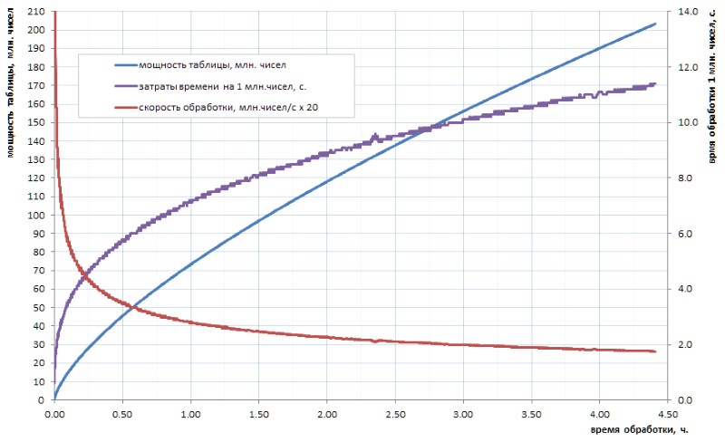
As can be seen from the diagram, the specific calculation time after the start-up jerk smoothly turns into asymptotic growth. It is rather slow. but this is growth, which means that the mining of each regular piece of data over time will be made more and more difficult. If you want to make some significant breakthrough, you have to parallelize the work on the cores (and it is well parallelized) and hang it on supercomputers. With the prospect of getting the first 10 billion simple in a week, and 100 billion - only in a year. Of course, there are faster algorithms for calculating simple ones than the trivial enumeration used in my homework, but, in essence, this does not change matters: after two or three orders of magnitude, the situation becomes similar.

So, it would be nice, once having done a counting job, to store its result in a ready-made tabular form, and use it as needed.

In view of the obviousness of the idea, there are a lot of links to ready-made lists of prime numbers that have already been calculated by someone. Alas, most of them are suitable only for student crafts: one such, for example, wanders from site to site and includes 50 million simple ones. This number can only amaze the uninitiated: it has already been mentioned above that on a home computer in a few hours you can independently calculate the table of all 32-bit simple ones, and it is four times more. Probably 15-20 years ago, such a list was indeed a heroic achievement for the non-professional community. Nowadays, in the age of multi-core multi-gigahertz and multi-gigabyte devices, this is no longer impressive.

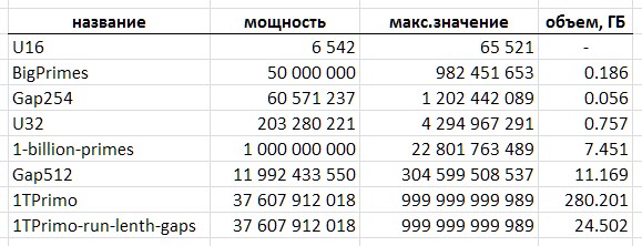
I was lucky to get an acquaintance access to a much more representative simple table, which I will continue to use as an illustration and sacrifice for my field experiments. In order to conspiracy call it 1TPrimo . It contains all the prime numbers less than a trillion.

Using the example of 1TPrimo, it is easy to see what volumes you have to deal with. With a capacity of about 37.6 billion values ​​in the format of 64-bit integers, this list takes 280 gigabytes. By the way - on that part of it, which could be packed in 32 bits, it is only 0.5% of the number of numbers represented in it. Whence it becomes absolutely clear that any serious work with prime numbers inevitably tends to total 64-bit (and more) bit depth.

Thus, the grim trend is obvious: a serious table of prime numbers inevitably has a titanic volume. And with this we must somehow fight.

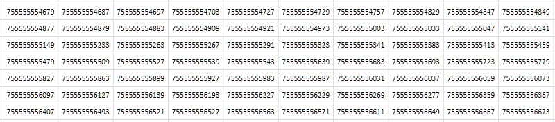
The first thing that comes to mind when looking at a table (Fig. 2) is that it consists of almost identical consecutive values ​​that differ only in the last one or two decimal places:

')

Simple, from the most common, abstract considerations: if there is a lot of duplicate data in the file, then it should be compressed well by the archiver. Indeed, the compression of the 1TPrimo table by the popular 7-zip utility with standard settings gave a rather high compression ratio: 8.5. True, the processing time - with the huge size of the source table - on an 8-core server, with an average load of all cores of the order of 80-90% was 14 hours and 12 minutes. Universal compression algorithms are designed for some abstract, generalized ideas about data. In some particular cases, specialized compression algorithms based on the well-known features of the incoming data set can demonstrate much more efficient performance, which is the subject of this work. And how effective - it will become clear below.

The close numerical values ​​of neighboring primes suggest the decision not to store these values ​​themselves, but the intervals (differences) between them. At the same time, it is possible to obtain substantial savings due to the fact that the width of the intervals is much lower than the width of the original data (Fig. 3).

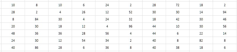
And it seems that it does not depend on the digit capacity of interval-generating simple ones. An "eye out" demonstrates that typical interval values ​​for primes taken from various places in the 1TPrimo table are within units, tens, occasionally hundreds, and - as a first working sentence - could possibly fit into the range of 8-bit unsigned integers, i.e., bytes. It would be very convenient, and in comparison with the 64-bit format, this would at once lead to 8-fold data compression - just somewhere at the level demonstrated by the 7-zip archiver. Moreover, the simplicity of the compression and decompression algorithms is supposed to have a profound effect on the speed of both compression and data access, compared to 7-zip. It sounds tempting.

At the same time, it is absolutely clear that the data converted from their absolute values ​​to relative intervals between them are suitable only for restoring series of values ​​that follow in succession from the very beginning of the table of primes. But if you add a minimum block-index structure to such a table of intervals, then with minor additional overhead costs this will allow you to restore — but block by block — both the table element by its number, and the closest element by an arbitrarily specified value, and these operations along with the main operation sampling of sequences in general exhausts the lion’s share of possible requests for such data. Of course, statistical processing will become more complicated, but nevertheless it will remain quite transparent, since There is no special trick in recovering it on the fly from the available intervals when accessing the required data block.

But alas. A simple numerical experiment on 1TPrimo data shows that already at the end of the third ten million (this is less than a hundredth percent of 1TPrimo volume) - and then everywhere - the intervals between adjacent simple ones regularly fall outside the range of 0..255.

Nevertheless, a slightly complicated numerical experiment reveals that the growth of the maximum interval between neighboring simple ones with the growth of the table itself goes very, very slowly - and this means that the idea is still good in some way.

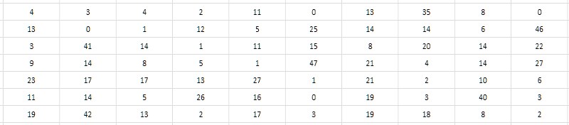
A second, closer look at the interval table suggests that you can store not the difference itself, but half of it. Since all primes greater than 2 are obviously odd, according to their differences they are obviously even. Accordingly, the differences can be reduced by 2 without losing the value; and for completeness, the unit can be subtracted from the obtained quotient in order to usefully dispose of the unclaimed otherwise zero value (Fig. 4). This coercion of intervals will be called further monolithic, in contrast to the friable, porous initial form, in which all odd values ​​and zero were unclaimed.

It should be noted that since the interval between the first two simple ones (2 and 3) does not fit into this scheme, then 2 will have to be excluded from the interval table and keep this fact in mind all the time.

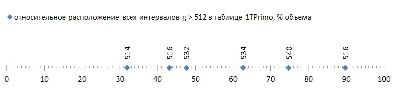
This simple technique allows to encode intervals from 2 to 512 in the range of values ​​of 0..255. Hope comes to life again that the difference method will allow to pack a much more powerful sequence of prime numbers. And rightly so: the run of 37.6 billion values ​​presented in the 1TPrimo list revealed only 6 (six!) Intervals that are not in the 2..512 range.

But it was good news; the bad thing is that these six intervals are scattered according to the list quite freely, and the first of them occurs already at the end of the first third of the list, turning the remaining two thirds into ballast unsuitable for this compression method (Fig. 5):

This kind of flush (some unfortunate six of them for almost forty billions! - and on you ...) even with a spoonful of tar to compare - honor of tar to show. But alas, this is a pattern, not an accident. If we trace the first occurrence of the intervals between primes depending on the bit depth of the data, it becomes clear that this phenomenon lies in the genetics of prime numbers, although it progresses extremely slowly (Fig.6 *).

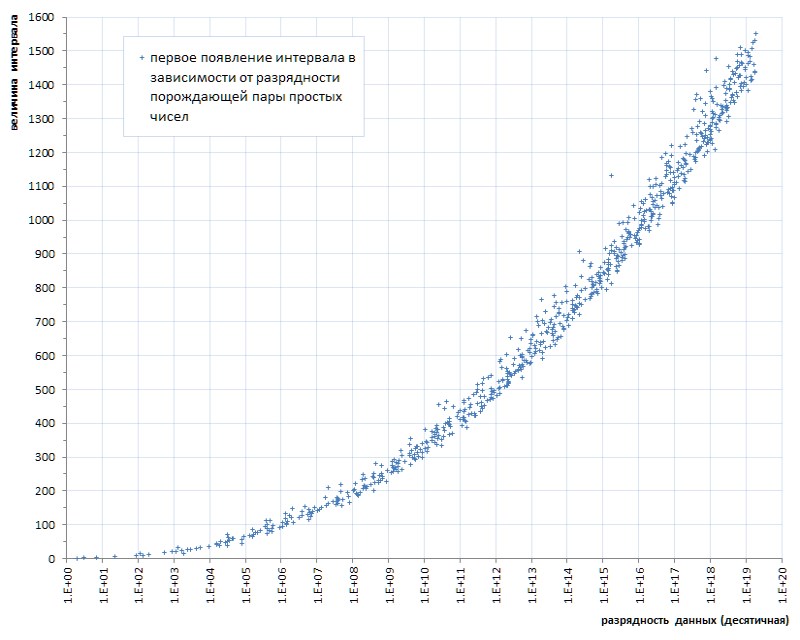
* The schedule is compiled according to the thematic website of Thomas R. Nicely ,
which are several orders higher than the power of the 1TPrimo list

But even this very slow progress unambiguously hints: it is possible to confine ourselves to some predetermined interval width only on some predetermined power of the list. That is, not suitable as a universal solution.

However, the fact that the proposed method of compressing a sequence of primes allows an uncomplicated compact table with a capacity of almost 12 billion values ​​to be realized - this is already quite an outcome. Such a table occupies a volume of 11.1 gigabytes - against 89.4 gigabytes in a trivial 64-bit format. Surely for a number of applications such a solution may be sufficient.

And what is interesting: the procedure for translating the 64-bit table 1TPrimo into the format of 8-bit intervals with a block structure, using only one processor core (for parallelization would have to resort to a significant complication of the program, and it was not worth it) and no more than 5 % of the processor load (most of the time was spent on file operations) took only 19 minutes. Against - let me remind you - 14 hours on eight cores with 80-90% of the load spent by the 7-zip archiver.

Of course, only the first third of the table was subjected to this broadcast, in which the range of intervals does not exceed 512. Therefore, if you bring the full 14 hours to the same third, then 19 minutes should be compared against almost 5 hours of the 7-zip archiver. With a comparable amount of compression (8 and 8.5), the difference is about 15 times. Taking into account that the lion's share of the working time of the broadcast program was taken by file operations, on a faster disk system the difference would be even steeper. And according to the mind, the running time of 7-zip on eight cores should be recalculated into one stream, and then the comparison will become really adequate.

A sample from such a database differs very little in time from a sample from a table of unpacked data and is almost entirely determined by the time of file operations. Specific figures are highly dependent on a specific hardware, on my server, on average, access to an arbitrary data block took 37.8 µs, with sequential reading of blocks - 4.2 µs per block, for full unpacking of the block - less than 1 µs. That is, comparing data unpacking with the work of a standard archiver does not make sense at all. And this is a big plus.

And finally, the observations made suggest another, third solution, which removes any limitations on data power: interval coding with variable length values. This technique has long been widely used in applications related to compression. Its meaning is that if in the input data it is found that some values ​​come across often, some less often, and some rarely come up, then we can encode the first with short codes, the second with longer codes, and the third - very long (maybe even very long, because it does not matter: all the same, such data is very rare). As a result, the total length of the received codes can be much shorter than the input data.

Already looking at the graph of the appearance of the intervals in Fig. 7, one can make an assumption that if the intervals are 2, 4, 6, etc. appear before the intervals, say, 100, 102, 104, etc., and then the first should occur much more often than the second. And vice versa - if the intervals 514 come across only from 11.99 billionths, 516 - starting from 16.2 billions, and 518 - generally starting only from 87.7 billions, then they will continue to fall very rarely. That is, a priori, we can assume an inverse relationship between the size of the interval and its frequency in the sequence of primes. So, it is possible to construct a simple structure that implements variable length codes for them.

Of course, the statistics of frequency of intervals should be decisive for choosing a specific coding method. Fortunately, in contrast to arbitrary data, the frequency of the intervals between prime numbers - which themselves are strictly deterministic, once and for all a given sequence - is also strictly deterministic, once and for all a certain characteristic.

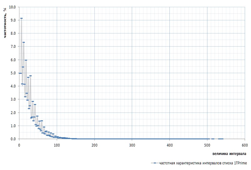
Figure 7 shows the frequency response of the intervals for the whole 1TPrimo list:

Here we must again mention that the interval between the very first simple 2 and 3 is excluded from the graph: this interval is equal to 1 and occurs in the sequence of simple exactly once, regardless of the power of the list. This interval is so distinctive that it is easier to remove 2 from the list of simple ones, than to constantly stumble upon reservations. Sim is declared that the number 2 is virtual simple : it is not visible in the lists, but it is there. Like that gopher.

At first glance, the frequency graph fully confirms the a priori assumption given by the pair of paragraphs above. It clearly shows the statistical heterogeneity of intervals and the high frequency of small values ​​compared with large ones. However, on the second, more convex view, the graph turns out to be much more interesting (Fig. 8):

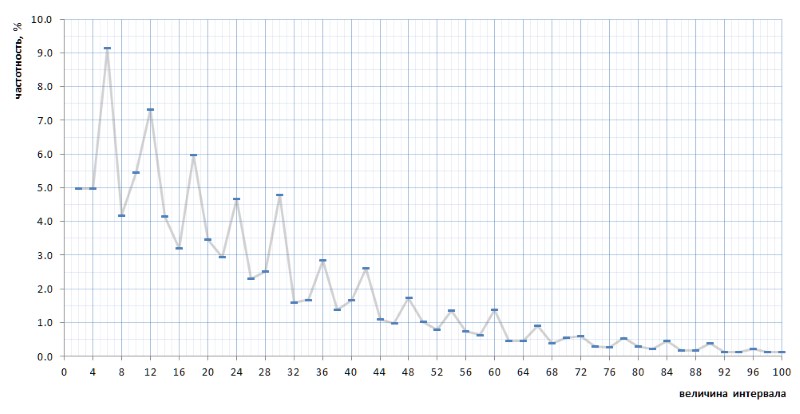
Quite unexpectedly, it turns out that the most common intervals are not 2 and 4, as it seemed to be from general considerations, but 6, 12 and 18, followed by 10 - and only then 2 and 4 with practically equal frequency (the difference in 7 after comma). And further multiplicity of peak values ​​of the number 6 is traced throughout the entire graph.

Even more interesting is that this inadvertently revealed nature of the schedule is universal - and, in all details, with all its kinks - throughout the sequence of simple intervals represented by the list of 1TPrimo, and there is a possibility that it is universal in general for any sequence of intervals of simple (of course such a bold statement needs proof, which I will with great pleasure transfer to the specialists in number theory). Figure 10 presents a comparison of the full statistics of the intervals (a line of scarlet) with limited sampling intervals taken at several arbitrary locations in the 1TPrimo list (lines of other colors):

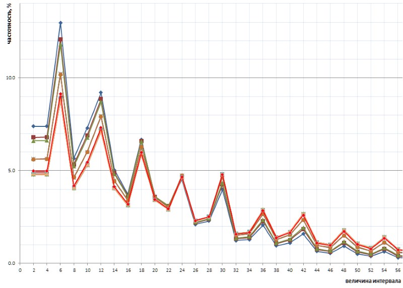
It can be seen from this graph that all these samples repeat each other exactly, with only a small difference in the left and right parts of the figure: they seem to be slightly rotated counterclockwise around the point of the interval with a value of 24. This rotation is probably due to the fact that the higher in the left parts of the graphics are built on samples with lower bit depth. In such samples there are still no, or rarely large intervals, which become frequent in the samples with higher bit depth. Accordingly, their absence is in favor of the frequency of intervals with smaller values. In samples with a higher bit depth, many new intervals appear with larger values, so the frequency of smaller intervals decreases slightly. Most likely, the turning point, with an increase in the power of the list, will shift towards larger values. Somewhere in the same place is the balance point of the graph, where the sum of all values ​​on the right is approximately equal to the sum of all values ​​on the left.

This entertaining nature of the frequency of intervals suggests discarding the trivial structure of variable-length codes. Usually such a structure consists of a packet of bits of various lengths and purposes. For example, first comes a certain number of prefix bits set to a specific value, for example, 0. They are followed by a stop bit, which should mark the end of the prefix, and, accordingly, must be different from the prefix: 1 in this case. The prefix may not have any length, that is, the sample may begin immediately with a stop bit, thus determining the shortest sequence. The stop bit is usually followed by a suffix, the length of which is determined in some pre-defined manner by the prefix length. It can be equal to the prefix length, it can be a specified number of times longer, or the dependence can be progressive - the choice is determined just by the frequency characteristics of the input data. Since the length of the suffix is ​​already defined by the prefix, the bits of the suffix can have any value and denote something. Thus, the suffix in some way predetermined way (tabular, calculated, some other) determines the value that should be restored from parsed packet of bit sequences.

In our case, the identified cyclical nature of the frequency response allows us to supplement the structure described above with another pendulum reflecting this cyclicity.

And here you should say another important thing. At first glance, the observed cyclicity implies dividing the intervals into triples: {2,4, 6 } , {8,10, 12 } , {14,16, 18 } and so on (the values ​​with the maximum frequency in each triples are highlighted in bold) . However, in reality the cyclicality here is slightly different.

I will not give the whole course of reasoning, of which, in fact, no: it was an intuitive guess, supplemented by a method of stupid searching variants, calculations and samples that took several days with interruptions. The resulting cyclicality consists of six intervals {2,4, 6 ,8,10, 12 } , {14,16, 18 ,20,22, 24 } , {26,28, 30 ,32,34, 36 } and so on (intervals of maximum frequency are highlighted in bold again).

In a nutshell, the proposed packaging algorithm is as follows.

The division of intervals into sixes of even numbers allows us to represent any interval g as g = i * 12 + t , where i is the index of the six that includes this interval ( i = {0,1,2,3, ...} ) t - scam representing one of the values ​​from a rigidly defined, bounded and identical set for any six {2,4,6,8,10,12} . The frequency response of the index highlighted above is almost exactly inversely proportional to its value, so it is logical to convert the six index into a trivial variable-length code structure, an example of which is given above. The frequency characteristics of the scraper allow us to divide it into two groups that can be encoded with bit chains of different lengths: values ​​6 and 12, which occur most often, encode with one bit, values ​​2, 4, 8 and 10, which occur much less frequently, encode with two bits. Of course, we need one more bit to distinguish these two options.

An array containing bit packets is supplemented with fixed fields that specify the starting values ​​of the data presented in the block, and other values ​​required to restore an arbitrary simple or sequence of simple intervals from the intervals stored in the block.

In addition to this block-index structure, the use of variable-length codes is complicated by additional costs compared to fixed-length intervals.

When using intervals of a fixed size, determining a block in which a prime number should be searched for by its ordinal number is a rather simple task, since the number of intervals per block is known in advance. But the search for a simple by the nearest value has no direct solution. Alternatively, you can use any empirical formula that allows you to find an approximate block number with the required interval, after which you will have to search for the desired block by searching.

For a table with variable length codes, the same approach is required for both tasks: both for sampling values ​​by number and for searching by value. Since the length of the codes varies, it is never known beforehand how many differences are stored in any particular block, and in which block the desired value lies. It was experimentally determined that with a block size of 512 bytes (which includes some number of bytes of the header), the capacity of the block can walk by 10-12 percent of the average value. Smaller blocks give even more relative scatter. At the same time, the average value of the block capacity itself tends to slow down as the table grows. Selection of empirical formulas for inaccurate determination of the initial block for finding the desired value, both by number and value, is a nontrivial task. Alternatively, you can use more complex and sophisticated indexing.

That's all.

Below, the subtleties of compression of the table of prime numbers using variable length codes and the structures associated with it are described more formally and in detail, the code for the functions of packing and unpacking intervals in the C language is given.

Total.

The amount of data translated from the 1TPrimo table to variable length codes, supplemented by a block-index structure, also described below, was 26,309,295,104 bytes (24.5GB), that is, the compression ratio reaches a value of 11.4. It is obvious that with the increase in the digit capacity of data the compression ratio will grow.

The broadcast time of 280 GB of the 1TPrimo table to the new format was 1 hour. This is an expected result after experiments with packing single-byte intervals. In both cases, the translation of the source table consists mainly of file operations and almost does not load the processor (in the second case, the load is still higher due to the higher numerical complexity of the algorithm). The data access time is also not much different from single-byte intervals, but the time to unpack a full block of the same size took 1.5 µs, due to the higher complexity of the algorithm for extracting variable length codes.

The table (fig.10) summarizes the volumetric characteristics of the primes table mentioned in this text.

Description of the compression algorithm

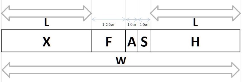
Terms and designations

P (prime): P1=3, P2=5, P3=7 ... Pn, Pn1 are prime numbers by their ordinal numbers. Once again (and last time) I emphasize that P0=2 is a virtual prime number; for the sake of formal uniformity, physically from the list of primes, this number is excluded.

G (gap) - the interval between two consecutive primes Gn = Pn1 - Pn; G={2,4,6,8 ...} Gn = Pn1 - Pn; G={2,4,6,8 ...} .

D (dense) - the interval reduced to a monolithic form: D = G/2 -1; D={0,1,2,3 ...} D = G/2 -1; D={0,1,2,3 ...} . The six intervals in the reduced to a monolithic form look like {0,1,2,3,4,5}, {6,7,8,9,10,11}, {12,13,14,15,16,17} etc.

Q (quotient) - an index of a six reduced to a monolithic form, Q = D div 6; Q={0,1,2,3 ...} Q = D div 6; Q={0,1,2,3 ...}

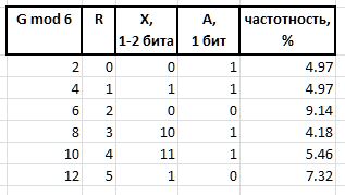
R (remainder) is the remainder of the monolithic six R = D mod 6. R always has a value in the interval {0,1,2,3,4,5} .

The values ​​of Q and R obtained by the above method from any arbitrary interval G , by virtue of their stable frequency characteristics, are subject to compression and storage in the form of bit packets of variable length, described below. Bit chains encoding Q and R values ​​in a packet are created in different ways: the bit chain of the prefix H , flux F and auxiliary bit S used to encode the Q index, and the bit group of the infix X and the auxiliary bit A are used to encode the remainder R

A (arbiter) is a bit that determines the size of the X infix: 0 is single-bit infix, 1 is two-bit.

X (infix) - 1 or 2-bit infix, together with the arbiter bit, reciprocally determining the value of R tabular manner (the table also shows the frequency of the first six with such infixes for reference):

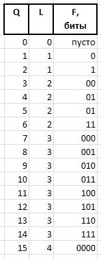
F (fluxion) is a fluxia, a derivative of the index Q variable length L={0,1,2...} , designed to distinguish between the semantics of bit chains (), 0, 00, 000, or 1, 01, 001 , and so on. d.

The bit chain of units of length L is expressed by the value 2^L - 1 (the sign ^ means exponentiation). In the notation of C, the same value can be obtained by the expression 1<<L - 1 . Then the value of the fluxion of length L can be obtained from Q expression

 F = Q - (1 << L - 1),

and restore Q from flux expression

 Q = (1 << L - 1) + F.

As an example, for the values Q = {0..15} , the following fluxium bit chains will be obtained:

The last two bit fields required for packing / retrieving values ​​are:

H (header) is a prefix, a string of bits set to 0.

S (stop) - stop bit set to 1, the final prefix.

In fact, these bits are processed first in the bit chains, they allow you to determine the size of the fluxion and the beginning of the arbitrator and fluxia when you unpack it or specify the packing immediately after the stop bit.

W (width) - the width of the entire code in bits.

The complete structure of the bit packet is shown in Figure 11:

The values ​​of Q and R restored from these chains allow us to restore the original value of the interval:

 D = Q * 6 + R,
 G = (D + 1) * 2,

and the sequence of restored intervals allows you to restore the original prime numbers from a given basic block value (seed block intervals) by adding to it sequentially all the intervals of this block.

To work with bit chains, a 32-bit integer variable is used in which the low-order bits are processed and, after using them, the bits are shifted to the left during packaging or to the right during decompression.

Block structure

In addition to bit chains, the block contains information necessary for sampling or for adding bits, as well as for determining the contents of a block.

 //      //    typedef unsigned char BYTE; typedef unsigned short WORD; typedef unsigned int LONG; typedef unsigned long long HUGE; typedef int BOOL; #define TRUE 1 #define FALSE 0 #define BLOCKSIZE (256) // :   , #define HEADSIZE (8+8+2+2+2) //   , #define BODYSIZE (BLOCKSIZE-HEADSIZE) //   . //           typedef struct { HUGE base; //  ,      HUGE card; //        WORD count; //      WORD delta; // base+delta =      WORD offset; //        BYTE body[BODYSIZE]; //    } crunch_block; //    ,   put()  get() crunch_block block; //       . // NB:  len/val  rev/rel     //  ,    ,   //    . static struct tail_t { BYTE len; //      S  A BYTE val; //  ,   A  - S BYTE rev; //    BYTE rel; //    } tails[6] = { { 4, 3, 2, 3 }, { 4, 7, 5, 3 }, { 3, 1, 0, 4 }, { 4,11, 1, 4 }, { 4,15, 3, 4 }, { 3, 5, 4, 4 } }; //             BOOL put(int gap) { // 1.      int Q, R, L; //   (),  (),   int val = gap / 2 - 1; Q = val / 6; R = val % 6; L = -1; // .., 0 - 1 val = Q + 1; while (val) { val >>= 1; L++; } //    L val = Q - (1 << L) + 1; //  val <<= tails[R].len; val += tails[R].val; //      val <<= L; //   L += L + tails[R].len; //    // 2.   val  L   buffer   put_index if (block.offset + L > BODYSIZE * 8) // !      return FALSE; Q = (block.offset / 8); //  ,      R = block.offset % 8; //     block.offset += L; //      block.count++; //     block.delta += gap; if (R > 0) //        { val <<= R; val |= block.body[Q]; L += R; } //     L = L / 8 + ((L % 8) > 0 ? 1 : 0); //     while (L-- > 0) { block.body[Q++] = (char)val; val >>= 8; } return TRUE; } //          int get_index; //         //      int get() { if (get_index >= BODYSIZE * 8) return 0; //      int val = *((int*)&block.body[get_index / 8]) >> get_index % 8; //  4   if (val == 0) return -1; // !       int Q, R, L, F, M, len; // , , , ,     L = 0; while (!(val & 1)) { val >>= 1; L++; } //  -     if ((val & 3) == 1) //       R = (val >> 2) & 1; //   else R = ((val >> 2) & 3) + 2; //   len = tails[R].rel; get_index += 2 * L + len; val >>= len; M = ((1 << L) - 1); //   F = val & M; //    Q = F + M; //   return 2 * (1 + (6 * Q + tails[R].rev)); //         } 

Enhancements

If you feed the resulting baseline intervals to the same 7-zip archiver, then after an hour and a half of intensive work on an 8-core server, he manages to compress the input file by almost 5%. That is, in the database of intervals of variable length, from the point of view of the archiver, there is still some redundancy. This means there is reason to speculate a little (in the good sense of the word) on the topic of further reducing data redundancy.

The principal determinism of the sequence of intervals between simple numbers allows one to make accurate calculations of the coding efficiency by one or another method. In particular, small (and rather chaotic) sketches made it possible to draw a fundamental conclusion about the advantages of coding sixes over triples, and about the advantages of the proposed method over trivial codes of variable length (fig.12):

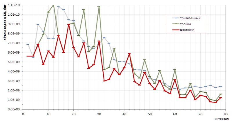
However, the annoying highs of the red graphics transparently hints that there may be other coding methods that would make the graph even flatter.

Another direction suggests checking the frequency of consecutive intervals. From general considerations: since the most common in the population of prime numbers are the intervals 6, 12, and 18, then they will probably also be more often found in pairs (doublets), triples (triplets), and similar combinations of intervals. If the repeatability of doublets (and maybe even triplets ... well, all of a sudden!) Turns out to be statistically significant in the total mass of intervals, then it will make sense to translate them into some separate code.

A full-scale experiment does reveal some predominance of individual doublets over others. However, if absolute leadership is expected in a pair (6,6) - 1.37% of all doublets - then the other winners of this rating are much less obvious:

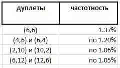
And since the doublet (6,6) symmetric, and all the remaining doublets are asymmetric and are found in the rating by mirror twins with the same frequency, it seems that the record record of the doublet (6,6) in this series should be divided in half between indistinguishable doubles (6,6) and (6,6) , which brings with them 0.68% far down, beyond the border of the prize list. And this once again confirms the observation that no true guesses regarding prime numbers are possible without surprises.

The statistics of triplets also demonstrates the leadership of such triples of intervals that do not quite fit into the speculative assumption emanating from the highest frequency of the intervals 6, 12, 18. In decreasing order of popularity, the leaders of the frequency among triplets are as follows:

etc.

I am afraid, however, that the results of my speculations will be of interest to not so much programmers, perhaps mathematicians, because of the unexpectedness of the proofs introduced by practice into intuitive guesses. It is unlikely that any significant dividend in favor of a further increase in the compression ratio will be able to squeeze the frequency out of the mentioned percentages, while the complexity of the algorithm threatens to grow very significantly.

Restrictions

It was already noted above that the growth of the maximum value of the intervals in connection with the digit capacity of primes is very, very slow. In particular, from Fig. 6, it can be seen that the interval between any prime numbers that can be represented in a 64-bit unsigned integer format will certainly be less than 1600.

The described implementation allows you to properly pack and unpack any 18-bit interval values ​​(in fact, the first packaging error occurs with an input interval of 442358). I do not have enough imagination to assume that the database of intervals of prime numbers is capable of growing to similar values: offhand it is somewhere around 100-bit integers, and it’s more accurate to calculate laziness. In the fire case, to expand the range of intervals at times will be easy.

Thank you for reading this place :)